Calculates variance partitioning for gllvm object with function VP() (alias varPartitioning()).
Function plotVarPartitioning() (alias plotVP() or just plot()) plots the results of variance partitioning of a fitted gllvm.
# S3 method for class 'gllvm'
VP(
  object,
  group = NULL,
  groupnames = NULL,
  adj.cov = TRUE,
  grouplvs = FALSE,
  calcr2scaled = FALSE,
  ...
)

# S3 method for class 'VP.gllvm'
print(x, ...)

plotVarPartitioning(
  x,
  main = "Variance Partitioning",
  xlab = "Response",
  ylab = "Variance proportion",
  legend.text = NULL,
  args.legend = list(cex = 0.7, x = "topright", bty = "n", inset = c(0, -0.15)),
  mar = c(4, 4, 6, 2),
  r2scaled = FALSE,
  ...
)

plotVP(x, ...)

# S3 method for class 'VP.gllvm'
plot(x, ...)
Arguments
- object
an object of class 'gllvm'.
- group
a vector of integers identifying grouping of X covariates, the default is to use model terms formula and lv.formula.
- groupnames
a vector of strings given as names for the groups defined in group
- adj.cov
logical, whether or not to adjust co-variation within the group
- grouplvs
logical, whether or not to group latent variables to one group
- calcr2scaled
logical, whether or not to also calculate r2 scaled variance partitioning. Defaults to FALSE. If true, squared correlation between data and predictions is used for continuous data (normal, gamma, exponent, beta, tweedie), squared spearman correlation for count and ordinal data, and Tjur's R2 for binary data. Note, interpret these cautiously.
- ...
additional graphical arguments passed to the barplot function
- x
a variance partitioning object for a gllvm produced by function varPartitioning.
- main
main title
- xlab
a label for the x axis.
- ylab
a label for the y axis.
- legend.text
a vector of names for the groups, as a default 'groupnames' from varPartitioning. If FALSE, legend not printed.
- args.legend
a list of additional arguments to pass to
legend().- mar
Margins of the plot. Default
c(4,4,6,2)- r2scaled
logical, whether or not to plot the response specific R2 -scaled variance partitioning. Defaults to FALSE.
Details
Variance for the linear predictor for response j can be calculated as
$$Var(\eta_j) = \sum_k \beta_{jk}^2*var(z_{.k}) + 2 \sum_{(k1=1,...,K-1)} \sum_{(k2=k1+1,...,K)} \beta_{j(k1)}\beta_{j(k2)} Cov(Z_{.k1},Z_{.k2}) , $$
where \(z_{.k}\) is a vector consisting of predictor/latent variable/row effect etc values for all sampling units i. If \(z_{.k}\)s are not correlated, covariance term is 0 and thus the variance explained of a response j for predictor \(z_{.k}\) is given as \(\beta_{jk}^2*var(z_{.k})/Var(\eta_j)\).
In case of correlated predictors, it is advised to group them into a same group. The variance explained is calculated for the correlated group of predictors together and adjusted with the covariance term.
Examples
# Extract subset of the microbial data to be used as an example
data(microbialdata)
X <- microbialdata$Xenv
y <- microbialdata$Y[, order(colMeans(microbialdata$Y > 0),
decreasing = TRUE)[21:40]]
fit <- gllvm(y, X[,1:3], formula = ~ pH + Phosp, family = poisson(),
studyDesign = X[,4:5], row.eff = ~(1|Site))
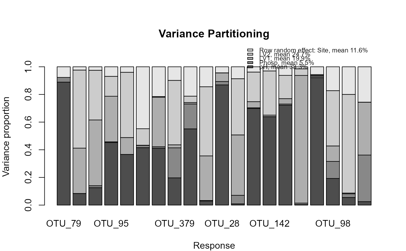
VP <- VP(fit)
plot(VP)
 if (FALSE) { # \dontrun{
# Plot the result of variance partitioning
plot(VP, col = palette(hcl.colors(5, "Roma")), las =2)
} # }
if (FALSE) { # \dontrun{
# Plot the result of variance partitioning
plot(VP, col = palette(hcl.colors(5, "Roma")), las =2)
} # }