Correlation structures for latent variables and row effects
Jenni Niku
2024-09-24
Source:vignettes/vignette9.Rmd
vignette9.RmdIn this example we demonstrate how to set correlation structures for latent variables and random effects in gllvm. The species abundances are often correlated in time or spatially in community ecology. In gllvm, such correlation structures can now be set either for latent variables or comunity level random row effects.
Denote the abundance of the th species () at the th site () as . A set of k environmental variables, or experimental treatments, may also be recorded at each site and stored in the vector . A common form for the GLLVM is then defined for the mean abundance :
Now we can specify a correlation structure for latent variables
(
number of latent variables, defined by num.lv in
gllvm) and/or community level row effects
.
The subscripts
defines the structure of the latent variables. For instance, assume that
we have a hierarchical sampling design with
sites and sites are sampled
times in consecutive years. Thus we could want to include a site level
latent variables such that
if sampling unit
is from site
().
Similarly, we can set a structure for the row effects defining subscript
,
eg. for time
if sampling unit
is from sampling year
().
Then we can define the correlation structures for latent variables
and/or row effects: denote
The covariance matrix
defines the correlation structure and has unit variances on diagonal.
The options are identity (independent), AR(1) correlation, exponentially
decaying correlation structure and Matern correlation. Currently we can
only use the same structure for all latent variables
,
but the parameters defining the strength of the correlation is estimated
uniquely for each latent variable.
Similarly, we can define the correlation structure for random row effect, denote , and set where the covariance matrix is a matrix and defines the correlation structure for random row effect. For row effects we have the same options as we have for latent variables. The structure for the row effects can be different from the structure of the latent variables and this is illustrated in the case study below.
As an example, we use time series of sessile algal and invertebrate species from permanent transects (Arkema et al. 2009, Reed and Miller (2023)). Data consists of percent cover of 132 species from 11 sites which each have 2-8 transects, yearly recorded from 2000 to 2021. It also includes measurements of the environment; the number of stripes of giant kelp and percent rock. In total, data has 836 sampling units.
data("kelpforest")
Yabund <- kelpforest$Y
Xenv <- kelpforest$X
SPinfo <- kelpforest$SPinfo
Species percent cover matrix is in Yabund, for the
analyses we consider only sessile invertebrates and include species
observed at least 10 times. The rarest species are modeled as a sum.
Yabund[1:10,1:20]## AB AL AMZO ANSP AR ARUD AS ATM AU BA BAEL BCAL BF BLD BN
## 1 0 0 0 0.0125 0 0 0.1125 0 0.0125 0.0000 0 0 0.0000 0 0.0125
## 2 0 0 0 0.0000 0 0 0.0000 0 0.0000 0.0000 0 0 0.0125 0 0.0000
## 3 0 0 0 0.0000 0 0 0.0750 0 0.0000 0.0000 0 0 0.0000 0 0.0000
## 4 0 0 0 0.0000 0 0 0.0125 0 0.0000 0.0000 0 0 0.0125 0 0.0000
## 5 0 0 0 0.0000 0 0 0.0000 0 0.0000 0.0000 0 0 0.0000 0 0.0000
## 6 0 0 0 0.0000 0 0 0.0000 0 0.0000 0.0000 0 0 0.0000 0 0.0000
## 7 0 0 0 0.0000 0 0 0.0000 0 0.0000 0.0000 0 0 0.0000 0 0.0000
## 8 0 0 0 0.0000 0 0 0.0000 0 0.0000 0.0000 0 0 0.0000 0 0.0000
## 9 0 0 0 0.0000 0 0 0.0500 0 0.0000 0.0125 0 0 0.0000 0 0.0000
## 10 0 0 0 0.0000 0 0 0.0250 0 0.0000 0.0000 0 0 0.0125 0 0.0000
## BO BOW BPSE BR BRA
## 1 0 0 0 0.0250 0.0375
## 2 0 0 0 0.0250 0.0125
## 3 0 0 0 0.0375 0.0000
## 4 0 0 0 0.0000 0.0000
## 5 0 0 0 0.0125 0.0000
## 6 0 0 0 0.0000 0.0125
## 7 0 0 0 0.0000 0.0000
## 8 0 0 0 0.0000 0.0000
## 9 0 0 0 0.1000 0.0000
## 10 0 0 0 0.1000 0.0875
Yinvert <- Yabund[SPinfo$GROUP == "INVERT"]
Yinvert10 = Yinvert[,colSums(Yinvert>0, na.rm = TRUE)>9]
# Sum species that were observed less than 9 times,
Yinvert10$Sum_inv = rowSums(Yinvert[,(colSums(Yinvert>0, na.rm = TRUE)<=9)], na.rm = TRUE)
There is information about the species:
head(SPinfo)## SP_CODE GROUP COMMON_NAME SCIENTIFIC_NAME TAXON_KINGDOM
## 1 AB INVERT Coarse Sea Fir Hydroid Abietinaria spp. Animalia
## 2 AL INVERT Aggregating cup Coral Astrangia haimei Animalia
## 3 AMZO ALGAE <NA> Amphiroa beauvoisii Plantae
## 4 ANSP INVERT Aggregating anemone Anthopleura spp. Animalia
## 5 AR INVERT Sand Tunicate Eudistoma psammion Animalia
## 6 ARUD INVERT Octocoral Discophyton rudyi Animalia
## TAXON_PHYLUM TAXON_CLASS TAXON_ORDER TAXON_FAMILY TAXON_GENUS
## 1 Cnidaria Hydrozoa Leptothecata Sertulariidae Abietinaria
## 2 Cnidaria Anthozoa Scleractinia Rhizangiidae Astrangia
## 3 Rhodophyta Florideophyceae Corallinales Lithophyllaceae Amphiroa
## 4 Cnidaria Anthozoa Actiniaria Actiniidae Anthopleura
## 5 Chordata Ascidiacea Aplousobranchia Polycitoridae Eudistoma
## 6 Cnidaria Anthozoa Alcyonacea Alcyoniidae Discophyton
SPinfo10 = SPinfo[SPinfo$SP_CODE %in% colnames(Yinvert10),]
SPinfo10 = rbind(SPinfo10,c("Sum_inv","INVERT", rep(NA, ncol(SPinfo10)-2)))
And finally, information about the study design (site name, year, transect index) and environmental coefficients (average number of kelp fronds, percent rock). The distribution of kelp fronds is very skewed to the right so a log of the number of kelp fronds is used as a covariate instead. In addition, covariates are scaled.
head(Xenv)## SITE YEAR TRANSECT KELP_FRONDS PERCENT_ROCKY
## 1 ABUR 2001 1 13.8750 35.0
## 2 ABUR 2001 2 0.0000 37.5
## 3 ABUR 2002 1 8.5125 10.0
## 4 ABUR 2002 2 0.3875 2.5
## 5 ABUR 2003 1 0.6000 0.0
## 6 ABUR 2003 2 0.0000 0.0
par(mfrow=c(1,2))
hist(Xenv$KELP_FRONDS, main = "KELP FRONDS")
Xenv$logKELP_FRONDS = log(Xenv$KELP_FRONDS+1)
Xenv$logKELP_FRONDSsc = scale(Xenv$logKELP_FRONDS)
Xenv$PERCENT_ROCKYsc = scale(Xenv$PERCENT_ROCKY)
hist(Xenv$logKELP_FRONDSsc, main = "log of KELP FRONDS")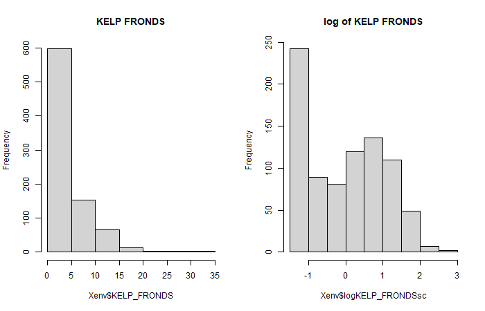
plot of chunk Xcovar
For modeling percent cover data, has three options, beta for values (0,1), ordered beta for [0,1] and beta hurdle model for [0,1). Here we use beta-hurdle response model.
Structured and correlated community level random row effects
The structure for community level row effects can be defined using
argument row.eff and defining the study design using
argument studyDesign. The structure is defined by common
formula interface; eg. row.eff = ~(1|site) and
site factor in a data.frame given in argument
studyDesign defines site level random effects. There are
four correlation structures available in , AR(1) corAR1,
compound symmetry corCS, exponentially decaying
corExp and Matern correlation corMatern. If
one would like to set eg. spatial correlation structure for the site
level random effects, it could be defined for instance by
row.eff = ~corExp(1|site) and spatial coordinates given to
dist as a matrix. Multiple row effect structures are
allowed.
In the next example, we attempt to model species abundances correlation in time using AR(1) correlated community level random effect for sampling year as well as site level row effects. Latent variables are left out from this model for now.
# Define the study design, now we need year and site
studyDesign = data.frame(year = factor(Xenv$YEAR), site = factor(Xenv$SITE))
# Set common shape parameter of beta distribution for different species (optional)
shapeForm = rep(1, ncol(Yinvert10))
# Fit model with AR(1) correlated random effect for sampling year
ftRowAR <- gllvm(Yinvert10, Xenv, family = "betaH",
                 formula = ~ logKELP_FRONDSsc + PERCENT_ROCKYsc,
                 studyDesign = studyDesign,
                 row.eff = ~ (1|site) + corAR1(1|year),
                 num.lv = 0, disp.formula = shapeForm)
ftRowAR## Call:
## gllvm(y = Yinvert10, X = Xenv, formula = ~logKELP_FRONDSsc +
## PERCENT_ROCKYsc, family = "betaH", num.lv = 0, studyDesign = studyDesign,
## row.eff = ~(1 | site) + corAR1(1 | year), disp.formula = shapeForm)
## family:
## [1] "betaH"
## method:
## [1] "VA"
##
## log-likelihood: -1448.781
## Residual degrees of freedom: 48907
## AIC: 3731.561
## AICc: 3738.689
## BIC: 7403.732If we look at the estimates, sd of the random effect for site is 0.106 and for year is 0.037 and AR(1) correlation between two consecutive years is 0.57. See below the parameter values and the row effects for years
# sds for random row effects and Correlation for consecutive years
ftRowAR$params$sigma
## site year yearrho
## 0.10601458 0.03676497 0.57861515
# Plot random effects and 95% predicted envelope
rowSite = ftRowAR$params$row.params[1:ftRowAR$grps.row["site"]]
years = matrix(as.numeric(levels(studyDesign$year)))
rowYear = ftRowAR$params$row.params[-(1:ftRowAR$grps.row["site"])]
# Calculate prediction errors for row effects:
predLVR = getPredictErr(ftRowAR)
# prediction errors for site effects
seSite = predLVR$row.effects[[1]]
# prediction errors for year effects
seYear = predLVR$row.effects[[2]]
# Plot:
par(mfrow=c(1,2))
plot(rowSite, ylim = range(rowSite) + c(-1.96,1.96)*max(abs(seSite)), main = "Random effect: site")
lines(rowSite - 1.96*seSite, col=2)
lines(rowSite + 1.96*seSite, col=2)
plot(years, rowYear, ylim = range(rowYear) + c(-1.96,1.96)*max(abs(seYear)), main = "Random effect: year")
lines(years, rowYear - 1.96*seYear, col=2)
lines(years, rowYear + 1.96*seYear, col=2)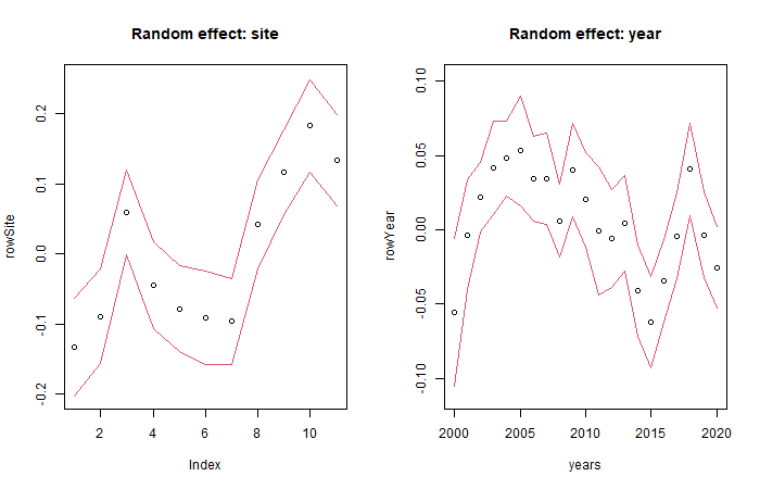
plot of chunk plotrow
The random effect for year represents the average trend of the all species abundances over the years which is not explained by the covariates.
To evaluate how much of the variation random effects and covariates are able to explain, calculate variance partitioning for the model. The random effect for year explains on average only 1.6% and the random effect for site 13.9% of the variation when modeling the probability of the presence, while conditional on the presence of the species, random year explains on average 5.9% and random site 52.5% of the variation of the coverage.
VP1 <- VP(ftRowAR)
plot(VP1, args.legend = list(cex=0.7), col=hcl.colors(5, "Roma"))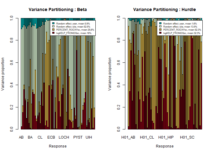
plot of chunk VP1
Structured and correlated latent variables
Structured latent variables
In the previous example, we did not include latent variables in the
model, but let’s focus on them now. Similarly to community level row
effects we can now set a structure for the latent variables as well
using argument lvCor. For instance, we could like to
account the variation in transects and sites and possible missing
environmental covariates that affect the species abundances. So let’s
include in the model also transect level latent variables, leave random
effect for site out:
# Define the study design, now we need year and site x transect
Xenv$STRANSECT =  factor(paste(Xenv$SITE,Xenv$TRANSECT, sep = ""))
studyDesign = data.frame(year = factor(Xenv$YEAR), stransect = factor(Xenv$STRANSECT))
# Fit model with AR(1) correlated random effect for sampling year
# and two transect level latent variable (two LVs model was better than 1 LV)
# Different starting values can be tested but zero starting values worked best in this case:
# (This can take a few minutes ~2-5)
ftRowAR_lv2 <- gllvm(Yinvert10, Xenv, family = "betaH",
                     formula = ~ logKELP_FRONDSsc + PERCENT_ROCKYsc,
                     studyDesign = studyDesign, row.eff = ~ corAR1(1|year),
                     num.lv = 2, lvCor = ~ (1|stransect),
                     disp.formula = shapeForm)
ftRowAR_lv2## Call:
## gllvm(y = Yinvert10, X = Xenv, formula = ~logKELP_FRONDSsc +
## PERCENT_ROCKYsc, family = "betaH", num.lv = 2, lvCor = ~(1 |
## stransect), studyDesign = studyDesign, row.eff = ~corAR1(1 |
## year), disp.formula = shapeForm)
## family:
## [1] "betaH"
## method:
## [1] "VA"
##
## log-likelihood: 793.3203
## Residual degrees of freedom: 48673
## AIC: -284.6406
## AICc: -267.1993
## BIC: 5448.174Below we plot the ordination, which is now at transect level, not sample level.
layout(matrix(c(1,2),1))
par(mar=c(4,4,3,1))
# Color code for sites
colSite = t(model.matrix(~studyDesign$stransect-1))%*% as.numeric(factor(Xenv$SITE))/colSums(model.matrix(~studyDesign$stransect-1))
# Ordination of sites+transect/Latent variables with 95% prediction regions
ordiplot(ftRowAR_lv2, predict.region = "sites", s.colors = colSite)

# Random effect for years:
years = matrix( as.numeric(levels(studyDesign$year)))
rowYear2 = ftRowAR_lv2$params$row.params
years = matrix( as.numeric(levels(studyDesign$year)))
predLVR = getPredictErr(ftRowAR_lv2)
plot(years, rowYear2, ylim = range(rowYear2) +
     c(-1.96,1.96)*max(abs(predLVR$row.effects[[1]])),
     main = "Random effect year", ylab = "")
lines(years, rowYear2 - 1.96*predLVR$row.effects[[1]], col=2)
lines(years, rowYear2 + 1.96*predLVR$row.effects[[1]], col=2)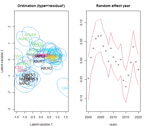
plot of chunk ordiplot1
The variance partitioning for the model shows that random effect for year explains on average only 0.6% of the variation when modeling the probability of the presence, while conditional on the presence of the species, random year explains on average 20.5% of the variation of the coverage. On the other hand, transect level latent variables can explain a total of 60% of the variation in presence-absence model, while for coverage model the proportion is smaller, around 40%.
VP2 <- VP(ftRowAR_lv2)
plot(VP2, args.legend = list(cex=0.7), col=hcl.colors(5, "Roma"))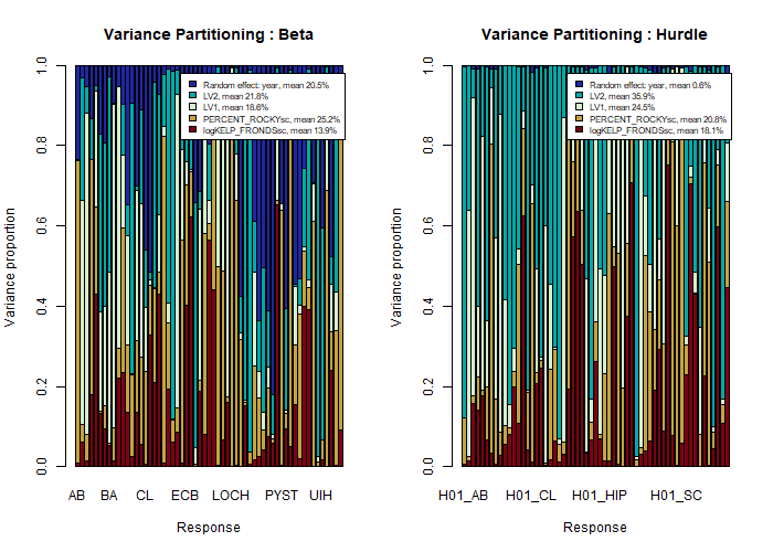
plot of chunk VP2
Correlated latent variables
It is also possible to specify a correlation structure for latent variables. An optimal choice would be to continue the analysis by setting spatial correlation structure for the sites or the transects, but the data do not have information about the coordinates. Instead, we illustrate this functionality below by setting AR(1) correlated latent variable for years. The variability between sites is now taken into account with random row effect.
Regarding the model estimation method, by default package uses
variational approximation (VA) method. VA-method approximates the
posterior distribution of the random effects and latent variables with
so called a variational covariance matrix. The structure of the
variational covariance can affect the accuracy of the method. For
example, an unstuctured variational covariance matrix (default) may lead
to more accurate results, but as a downside, it can be slow. If the
number of correlated levels, eg. sites or time points, is small, it does
not matter that much which structure is chosen, but for large number of
correlated levels the difference in computation time may be significant.
For correlated LVs there are few different options, as a alternatives to
the default choice we suggest either Lambda.struc = "bdNN"
or Lambda.struc = "UNN" methods (these are the same if
number of correlated LVs is 1). The complexity of those structures can
be modified with argument NN which can be between 2 and the
number of levels of the variable defining correlation structure -1 (eg.
number of spatially correlated sites -1 or number of correlated time
points -1). For this example, we set Lambda.struc = "bdNN"
and NN=5.
# Check first the number of correlated levels:
levels(studyDesign$year)
# Number of levels = number of years = 21, so NN can be at most 21-1 = 20
# And then bdNN structure would be same as unstructured variational covariance matrix
# In the example below, we set NN = 5. For this example,
# larger number does not improve the model fit anymore.
# Fit model with AR(1) correlated latent variables for sampling year
# and transect level random row effect
# (This can take a few minutes)
system.time(ftRow_lv1AR <- gllvm(Yinvert10, Xenv, family = "betaH",
                     formula = ~ logKELP_FRONDSsc + PERCENT_ROCKYsc,
                     studyDesign = studyDesign, row.eff = ~ (1|stransect),
                     num.lv = 1, lvCor = ~ corAR1(1|year),
                     Lambda.struc = "bdNN", NN=5, diag.iter = 0,
                     disp.formula = shapeForm))
ftRow_lv1AR## Call:
## gllvm(y = Yinvert10, X = Xenv, formula = ~logKELP_FRONDSsc +
## PERCENT_ROCKYsc, family = "betaH", num.lv = 1, lvCor = ~corAR1(1 |
## year), studyDesign = studyDesign, row.eff = ~(1 | stransect),
## disp.formula = shapeForm, Lambda.struc = "bdNN", NN = 5,
## diag.iter = 0)
## family:
## [1] "betaH"
## method:
## [1] "VA"
##
## log-likelihood: -922.7426
## Residual degrees of freedom: 48790
## AIC: 2913.485
## AICc: 2925.196
## BIC: 7615.978
# Correlation for consecutive years (LV)
ftRow_lv1AR$params$rho.lv
## rho.lv1
## 0.9046357
# sd of random row effects for transects
ftRow_lv1AR$params$sigma
## stransect
## 0.1433812The correlation for consequtive years is strong 0.90. Below we view the species specific yearly trends in the products of latent variables and loadings.
layout(matrix(c(1,2),1))
par(mar=c(4,4,3,1))
# When variation between sites was taken into account, there is no clear common trend
LVloadings = ftRow_lv1AR$lvs%*%t(ftRow_lv1AR$params$theta%*%diag(ftRow_lv1AR$params$sigma.lv,1))

years = matrix( as.numeric(levels(studyDesign$year)))
matplot(years, LVloadings[,1:ncol(Yinvert10), drop=FALSE], type = "l", ylab = "LV*Loadings", main = "Beta")
matplot(years, LVloadings[,-(1:ncol(Yinvert10)), drop=FALSE], type = "l", ylab = "LV*Loadings", main = "Hurdle")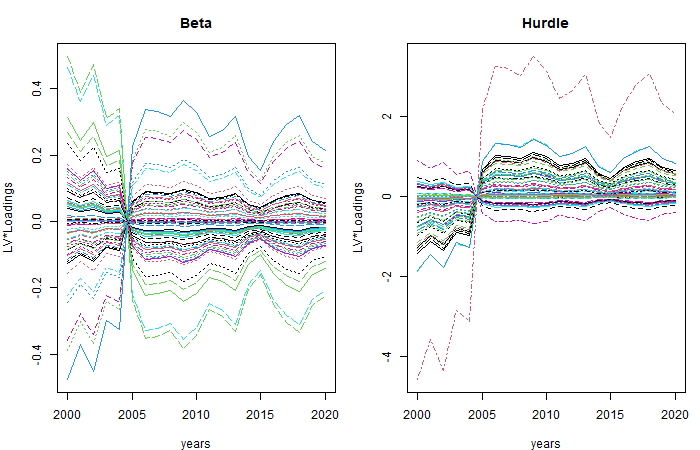
plot of chunk lvAR