Phylogenetic random effects
Bert van der Veen
2024-10-02
Source:vignettes/vignette7.Rmd
vignette7.RmdThis vignette is divided into two parts, the first part related to models with environment covariates only, and the second part for models that additionally incorporate trait covariates, so called “fourth corner” models. This is for convenience, as the interface for fitting fourth corner models slightly differs from the models without traits. Both models are detailed in van der Veen and O’Hara (2024), and the fourth corner model in more detail in Niku et al. (2021).
For more information about fitting trait models with random effects, see also vignette 1.
Phylogenetically structured environmental responses
In this vignette we demonstrate how to fit models that incorporate phylogenetic information into the random effects. For this, we make use of an adjusted version of the familiar lme4-formula interface Douglas Bates et al. (2024).
Here, we will use the data by Abrego et al. (2015). It includes information of 215 fungal species at 1666 European beech logs, and was analyzed by the original authors using a similar model. We start by loading the data:
library(gllvm)

data(fungi)
Y <- fungi$Y
X <- fungi$X
tree <- fungi$tree # the tree
colMat <- fungi$C # e.g., from ape::vcv(tree)
dist <- fungi$dist # e.g., from ape::cophenetic.phylo(tree)

# Scale the predictors
covs <- c("DBH.CM","AVERDP","CONNECT10","TEMPR","PRECIP","log.AREA")
X[,covs] <- scale(X[, covs])
The included version of the package does not contain all available environmental covariates, only those used in the original analysis. This includes diameter at breast height (DBH.CM), decay stage (AVERDP), connectivity of the surrounding forest (CONNECT10), annual temperature range, annual precipitation, and the logarithm of the reserve’s area.
We can think of the model as having two covariance matrices: one with correlation between covariate effects, and another that incorporates the correlation between species due to the phylogeny. The former is specified via the formula interface, the form of the latter is (more or less) fixed at present.
Species ordering
It is important to note that the error of the NNGP approximation that is used for fitting the models depends somewhat on the order of the species in the data (Guinness 2018). The software can minimize the number of VA parameters necessary by utilizing block structure in the phylogeny (i.e., full independence due to top splits), so the ideal ordering is often that provided by the tip labels in the phylogeny (so make sure not to arbitrarily order the response data). The VA method in the gllvm package retains block structure of the phylogenetic covariance matrix. This is not necessarily optimal in terms of approximation error of the NNGP.
A less than ideal ordering requires a larger number of nearest
neighbours for an accurate approximation. For cases when the ordering in
from the phylogenetic tree seems to function poorly, we provide a
function (note, not exported) in the package to help evaluate the error
due to a certain species ordering findOrder(). This
calculates the Frobenius norm of the product of the sparse approximation
to the inverse of the phylogenetic covariance matrix and the
phylogenetic covariance matrix, minus the identity matrix, given a
species order and number of nearest neighbours. It returns the error,
the approximation, and the ordering (which retains the block structure
if withinBlock = TRUE, the default). In short: a lower
error means a better approximation (but note the trade-off). Here is
some code to demonstrate this:
# order of species in phylogeny tips
# with a plot of error vs. nearest neighbours
err1 <- NULL
for(i in 1:215){
approx1 <- gllvm:::findOrder(covMat = colMat, distMat = dist, nn = i)
err1 <- c(err1, approx1$err)
}
plot(y=err1,x=1:215,type="l", xlab = "Neighbours", ylab = "Approximation error")
abline(v = 10, col = "red", lty = "dotted")
abline(v = 15, col = "red", lty = "dashed")
abline(v = 20, col = "red")

# order species alphabetically
err2 <- NULL
for(i in 1:215){
approx2 <- gllvm:::findOrder(covMat = colMat, distMat = dist, nn = i, order = order(tree$tip.label))
err2 <- c(err2, approx2$err)
}
lines(y=err2,x=1:215,col="blue")

# order species by sum of distances
order = order(colSums(dist),decreasing=TRUE)
err3 <- NULL
for(i in 1:215){
approx3 <- gllvm:::findOrder(covMat = colMat, distMat = dist, nn = i, order = order)
err3 <- c(err3, approx3$err)
}
lines(y=err3,x=1:215,col="forestgreen")

# order species by distance to the root
allDists <- ape::dist.nodes(tree)
err4 <- NULL
for(i in 1:215){
approx4 <- gllvm:::findOrder(covMat = colMat, distMat = dist, nn = i, order = as.integer(names(sort(allDists[1:length(tree$tip.label), nrow(allDists)],decreasing = TRUE))))
err4 <- c(err4, approx4$err)
}
lines(y=err4,x=1:215,col="pink")

# order by internal order of edges
# order <- ape::reorder.phylo(tree, order = "postorder", index.only=TRUE)
# err5 <- NULL
# for(i in 1:215){
# approx5 <- gllvm:::findOrder(covMat = colMat, distMat = dist, nn = i, order = order[order<=length(tree$tip.label)])
# err5 <- c(err5, approx5$err)
# }
# lines(y=err5,x=1:215,col="purple")
#
# order <- ape::reorder.phylo(tree, order = "pruningwise", index.only=TRUE)
# err6 <- NULL
# for(i in 1:215){
# approx6 <- gllvm:::findOrder(covMat = colMat, distMat = dist, nn = i, order = order[order<=length(tree$tip.label)])
# err6 <- c(err6, approx6$err)
# }
# lines(y=err6,x=1:215,col="grey")

# by first eigenvector
err7 <- NULL
order=order(eigen(colMat)$vec[,1],decreasing=TRUE)
for(i in 1:215){
approx7 <- gllvm:::findOrder(covMat = colMat, distMat = dist, nn = i, order = order)
err7 <- c(err7, approx7$err)
}
lines(y=err7,x=1:215,col="green")

# squared covariances
order = order(sapply(1:215,function(i, colMat)sum(colMat[i,][-1]^2), colMat = colMat),decreasing=FALSE)
err8 <- NULL
for(i in 1:215){
    approx8 <- gllvm:::findOrder(covMat = colMat, distMat = dist, nn = i, order = order)
    err8 <- c(err8, approx8$err)
}
lines(y=err8,x=1:215,col="brown")

# order by the distance of the n nearest neighbours
err9 <- NULL
for(i in 1:215){
    order = order(sapply(1:215,function(j,dist,nn)sum(dist[j,-j][order(dist[j,-j],decreasing=FALSE)[1:nn]]),nn=i,dist=dist),decreasing=TRUE)
    approx9 <- gllvm:::findOrder(covMat = colMat, distMat = dist, nn = i, order = order)
    err9 <- c(err9, approx9$err)
}
lines(y=err9,x=1:215,col="orange")

# minium sum to preceding species
#get colMat blocks first
p=215
blocks = list()
  B = 1
  E = B
  while(B<=p){
    while(E<p && (any(colMat[(E+1):p,B:E]!=0)|any(colMat[B:E,(E+1):p]!=0))){
      # expand block
      E = E+1;
    }
    # save block
    blocks[[length(blocks)+1]] = colMat[B:E,B:E,drop=FALSE]
    E = E+1;
    B = E;
  }
  err10 <- NULL
for(i in 1:215){
  ord <- NULL
  blocksp <- 0
  for(k in 1:length(blocks)){
    idx <- 1:nrow(blocks[[k]])
    ordnew <- which.max(apply(blocks[[k]],2,max))
    idx <- idx[idx!=ordnew]
for(l in 2:nrow(blocks[[k]])){
  #add entry of next species with min(i,nn) largest neighbour entries
  spec <- idx[which.min(sapply(idx,function(j,nn){
    x <- sum(blocks[[k]][ordnew,j])
    # x <- x[x!=0]
    # sum(x[order(x,decreasing=TRUE)[1:min(i,nn)]])
  }, nn = i))]
  ordnew <- c(ordnew,spec)
  idx <- idx[idx!=spec]
}
    ord <- c(ord, ordnew+blocksp)
    blocksp <- blocksp + nrow(blocks[[k]])
  }

approx10 <- gllvm:::findOrder(covMat = colMat, distMat = dist, nn = i, order = ord)
err10 <- c(err10, approx10$err)
}
lines(1:215,err10, col="purple")

# species with minimum of maximum distance to preceding species
# similar to algorithm maxmin from guiness2018?
p=215
blocks = list()
  B = 1
  E = B
  while(B<=p){
    while(E<p && (any(colMat[(E+1):p,B:E]!=0)|any(colMat[B:E,(E+1):p]!=0))){
      # expand block
      E = E+1;
    }
    # save block
    blocks[[length(blocks)+1]] = colMat[B:E,B:E,drop=FALSE]
    E = E+1;
    B = E;
  }
  err11 <- NULL
for(i in 1:215){
  ord <- NULL
  blocksp <- 0
  for(k in 1:length(blocks)){
    idx <- 1:nrow(blocks[[k]])
    ordnew <- which.max(apply(blocks[[k]],2,max))
    idx <- idx[idx!=ordnew]
for(l in 2:nrow(blocks[[k]])){
  #add entry of next species with min(i,nn) largest neighbour entries
  spec <- idx[which.min(sapply(idx,function(j,nn){
    x <- max(blocks[[k]][ordnew,j])
    # x <- x[x!=0]
    # sum(x[order(x,decreasing=TRUE)[1:min(i,nn)]])
  }, nn = i))]
  ordnew <- c(ordnew,spec)
  idx <- idx[idx!=spec]
}
    ord <- c(ord, ordnew+blocksp)
    blocksp <- blocksp + nrow(blocks[[k]])
  }

approx11 <- gllvm:::findOrder(covMat = colMat, distMat = dist, nn = i, order = ord)
err11 <- c(err11, approx11$err)
}
lines(1:215,err11, col="grey")


legend("topright", legend=c("Tips","Alphabetical", "Total distance", "Distance to root", "First eigenvector","Sum of squared covariances","Total distance (nn)", "minsum", "maxmin"), col=c("black","blue", "forestgreen","pink", "green", "brown","orange","purple","grey"),lty = rep("solid",9))
plot of chunk specord
#low number of neighbours: 3 is best.
#plot(y=apply(cbind(err1,err2,err3,err4,err7,err8,err9,err10,err11),1,which.min),x=1:215)
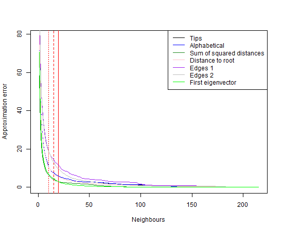
The red lines indicate 10, 15, and 20 neighbours. Clearly, ordering the species by the sum of distances, sum of squared covariances, or by the first eigenvector of the phylogenetic covariance matrix, give good approximations (i.e., most accurate with least neighbours) for this dataset.
This serves to demonstrate that the species order does matter to the approximation, and a better order may be available. In the plot we can see that the error reduces quickly towards 10-15 neighbours, and levels out after about 50 neighbours. If we plotted the same curve wit the computation time, it would probably exhibit the opposite of the displayed pattern.
Fit the model
TMB::openmp(parallel::detectCores()-1, autopar = TRUE) # set parallel computation
order <- gllvm:::findOrder(covMat = colMat, distMat = dist, nn = 15,
          order = as.integer(names(sort(allDists[1:length(tree$tip.label), nrow(allDists)],decreasing = TRUE))))$order
order <- tree$tip.label[order]
model1 <- gllvm(y = Y[,order], X = X,
        formula = ~(DBH.CM + AVERDP + I(AVERDP^2) + CONNECT10 + TEMPR + PRECIP + log.AREA|1), beta0com = TRUE,
                     family = "binomial", num.lv = 0, sd.errors = FALSE,
                     studyDesign = X[,c("REGION", "RESERVE")], row.eff = ~(1 | REGION/RESERVE),
                     colMat = list(colMat[order,order], dist = dist[order,order]), colMat.rho.struct = "term", nn.colMat = 15,
        optim.method = "L-BFGS-B")
Let’s walk through some of the specified arguments.
The first line enables parallel computation, to speed up model fitting.
Note that an intercept term is included in the random effects, which
can be excluded by incorporating a zero in the formula term.
Correlations are included between covariates inside the brackets, so we
could have uncorrelated effects by including them all in separately
bracketed terms. We specify num.lv = 0 for now, although we
could just as well include latent variables (e.g., we could fit a model
with phylogenetically structured random intercepts and a (un)constrained
ordination), and beta0comm to have a single (fixed)
intercept for the whole community (species-specific intercepts enter via
the random effects). sd.errors is here for convenience set
to false, as it can take a (much) longer time to calculate standard
errors than to fit the model, and we should really only calculate the
standard errors when we need them (e.g., for visualization). The
gllvm::se.gllvm function can post-hoc calculate the
standard errors, so that we do not need to refit the model.
The studyDesign matrix is specified to additionally
incorporated random intercepts for the nested study design. and a
formula row.eff to specify the random intercept structure.
The colMat term is how we pass the phylogenetic information
to the model, which is usually a list of length two, where one argument
is called dist and the other is the covariance matrix from
the tree. Note that these two matrices need to have the same column
names as Y. nn.colMat is the number of nearest
neighbours to consider for each species on the tree, which is fixed to
10 by default. Smaller numbers usually result in a faster fitting model,
but one that is potentially less accurate. van
der Veen and O’Hara (2024) showed that 10-15 neighbours is
usually a good choice, although fewer/more also still lead to accurate
estimates for the phylogenetic signal, but this can be quite problem
dependent. colMat.rho.struct has two options,
single fitting a model with the same phylogenetic signal
parameter for all covariates (default) and term fitting a
model with a phylogenetic signal parameter per covariate. Finally, the
last line changes the optimisation method to one that seems to usually
do well with this model type, and changes the starting values of the
random effect (which was needed to fit this model succesfully).
After model fitting, the random effect estimates can be found in
model1$params$Br, and prediction errors can be extracted
with gllvm::getPredictErr. This requires the standard
errors, so let’s calculate thosefirst:
# calculate standard errors
ses <- se.gllvm(model1) # this can take a few minutes
model1$sd <- ses$sd
model1$Hess <- ses$Hess
Here is some code to visualize the model results (from van der Veen and O’Hara (2024)):
# Making the term namees a bit prettier
row.names(model1$params$Br) <- c("Intercept", "Deadwood size", "Decay stage", "Decay stage²", "Connectivity", "Temperature range", "Precipitation","ln(Reserve area)")
model1$params$B[names(model1$params$B)%in%row.names(model1$params$Br)] <- row.names(model1$params$Br)[-1]
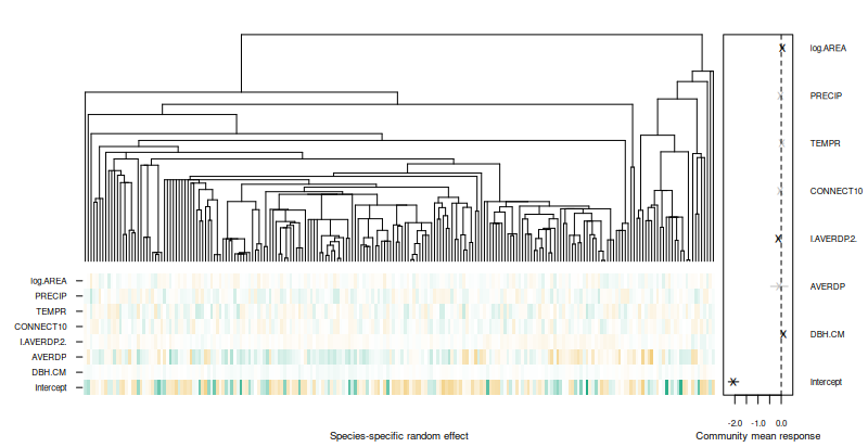
phyloplot(model1, tree)
plot of chunk bigplot
The random effects with a prediction interval including zero are
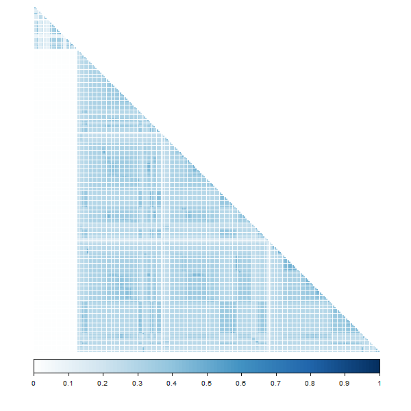
crossed out in the plot. The getResidualCov and
getResidualCor functions extract the residual covariance
and correlation matrix, respectively, for visualizing species
associations.
corrplot::corrplot(getEnvironCor(model1),
                   type = "lower", diag = FALSE, order = "AOE",
                   tl.pos = "n", addgrid.col=NA, col.lim=c(0,1))
plot of chunk corrplot
The randomCoefPlot function constructs caterpillar plots
of species deviations from the community mean responses, which can be
extracted via the summary method, or found via coef and in
model1$params$B.
Arguments to control the VA approximation are Ab.struct
and Ab.struct.rank, for details see van der Veen and O’Hara (2024). NOTE: Use
Ab.struct = "CL1" or Ab.struct="CL2" only in
parallel when using TMB::openmp(.., autopar=TRUE). Without
TMB’s “automatic” parallelization feature, memory use is excessively and
your computer will probably run out of memory (for a moderately large
number of sites and species) so that your R session will crash.
Finally, we can look at the summary information of the model:
summary(model1)##
## Call:
## gllvm(y = Y[, order], X = X, formula = ~(DBH.CM + AVERDP + I(AVERDP^2) +
## CONNECT10 + TEMPR + PRECIP + log.AREA | 1), family = "binomial",
## num.lv = 0, studyDesign = X[, c("REGION", "RESERVE")], colMat = list(colMat[order,
## order], dist = dist[order, order]), colMat.rho.struct = "term",
## row.eff = ~(1 | REGION/RESERVE), sd.errors = FALSE, beta0com = TRUE,
## nn.colMat = 15, optim.method = "L-BFGS-B")
##
## Family: binomial
##
## AIC: 103080 AICc: 103080 BIC: 103662.6 LL: -51486 df: 54
##
## Informed LVs: 0
## Constrained LVs: 0
## Unconstrained LVs: 0
##
## Formula: ~(DBH.CM + AVERDP + I(AVERDP^2) + CONNECT10 + TEMPR + PRECIP + log.AREA | 1)
## LV formula: ~ 0
##
## Random effects:
## Name Signal Variance Std.Dev Corr
## Intercept 0.2106 0.5218 0.7224
## DBH.CM 0.5031 0.0052 0.0722 0.7524
## AVERDP 0.9711 0.3825 0.6185 0.1015 -0.0181
## I.AVERDP.2. 0.8007 0.0122 0.1105 -0.4874 -0.4696 -0.4871
## CONNECT10 0.0613 0.0270 0.1642 -0.1800 -0.1082 0.1563 -0.1128
## TEMPR 0.0499 0.0436 0.2087 -0.1579 -0.2858 -0.0683 0.7212 0.3666
## PRECIP 0.0000 0.0324 0.1799 0.2290 0.6520 -0.3145 0.0977 -0.5629
## log.AREA 0.0310 0.0158 0.1258 -0.1418 -0.1302 0.0928 -0.6283 0.4803
##
##
##
##
##
##
##
## -0.2123
## -0.5604 -0.5228
##
## Coefficients predictors:
## Estimate Std. Error z value Pr(>|z|)
## Intercept -2.05756 0.13590 -15.140 < 2e-16 ***
## DBH.CM 0.10583 0.01936 5.465 4.62e-08 ***
## AVERDP -0.08548 0.22763 -0.376 0.707278
## I.AVERDP.2. -0.12467 0.03344 -3.728 0.000193 ***
## CONNECT10 -0.03260 0.04141 -0.787 0.431209
## TEMPR 0.03646 0.04454 0.818 0.413120
## PRECIP -0.02091 0.03726 -0.561 0.574756
## log.AREA 0.05643 0.02976 1.896 0.057952 .
## ---
## Signif. codes: 0 '***' 0.001 '**' 0.01 '*' 0.05 '.' 0.1 ' ' 1which gives us an overview of the community mean responses, as well
as the variance and correlation of random effects, and the phylogenetic
signal parameter in the column signal. This parameter
ranges between zero and one, at zero the species responses are not
phylogenetically structured, and at one they are fully phylogenetically
structured.
Phylogenetic fourth corner model
The fourth corner model extends the previous model with functional traits. The interface is still a little difference, so that correlation between random effects are always included. Otherwise the tools are similar, so we just present some example code here for fitting such a model, but do not discuss it further (see other vignettes in the gllvm R-package for discussion of the fourth corner model).
TR <- fungi$TR # the functional traits

model2 <- gllvm(y = Y, X = cbind(int = 1, X), TR = TR,
                     formula = ~DBH.CM + AVERDP + I(AVERDP^2) + CONNECT10 +
  TEMPR + PRECIP + log.AREA + (DBH.CM + AVERDP + I(AVERDP^2) + CONNECT10 + TEMPR + PRECIP + log.AREA):(PC1.1 + PC1.2 + PC1.3),
                      family = "binomial", num.lv = 0, studyDesign = X[, c("REGION", "RESERVE")],
                      colMat = list(C, dist = dist),
                      colMat.rho.struct = "term", row.eff = ~(1 | REGION/RESERVE), sd.errors = FALSE,
                      randomX = ~int + DBH.CM + AVERDP + I(AVERDP^2) + CONNECT10 + TEMPR + PRECIP + log.AREA,
                      beta0com = TRUE, Ab.struct = "MNunstructured", nn.colMat = 10, max.iter = 20000, maxit = 20000, optim.method = "L-BFGS-B",
randomX.start = "res")