Fits generalized linear latent variable model for multivariate data. The model can be fitted using Laplace approximation method or variational approximation method.
gllvm(
  y = NULL,
  X = NULL,
  TR = NULL,
  data = NULL,
  formula = NULL,
  family,
  num.lv = NULL,
  num.lv.c = 0,
  num.RR = 0,
  lv.formula = NULL,
  lvCor = NULL,
  studyDesign = NULL,
  dist = list(matrix(0)),
  distLV = matrix(0),
  colMat = NULL,
  colMat.rho.struct = "single",
  corWithin = FALSE,
  corWithinLV = FALSE,
  quadratic = FALSE,
  row.eff = FALSE,
  sd.errors = TRUE,
  offset = NULL,
  method = "VA",
  randomB = FALSE,
  randomX = NULL,
  beta0com = FALSE,
  zeta.struc = "species",
  plot = FALSE,
  link = "probit",
  Ntrials = matrix(1),
  Power = 1.1,
  seed = NULL,
  scale.X = TRUE,
  return.terms = TRUE,
  gradient.check = FALSE,
  disp.formula = NULL,
  control = list(reltol = 1e-10, reltol.c = 1e-08, TMB = TRUE, optimizer = ifelse((num.RR
    + num.lv.c) <= 1 | randomB != FALSE, "optim", "alabama"), max.iter = 6000, maxit =
    6000, trace = FALSE, optimizer.trace = 0, optim.method = NULL, nn.colMat = 10,
    colMat.approx = "NNGP"),
  control.va = list(Lambda.struc = "unstructured", Ab.struct = ifelse(is.null(colMat),
    "blockdiagonal", "MNunstructured"), Ab.struct.rank = 1, Ar.struc = "diagonal",
    diag.iter = 1, Ab.diag.iter = 0, Lambda.start = c(0.3, 0.3, 0.3), NN = 10),
  control.start = list(starting.val = "res", n.init = 1, n.init.max = 10, jitter.var = 0,
    jitter.var.br = 0, start.fit = NULL, start.lvs = NULL, randomX.start = "res",
    quad.start = 0.01, start.struc = "LV", scalmax = 10, MaternKappa = 1.5, rangeP =
    NULL, zetacutoff = NULL, start.optimizer = "nlminb", start.optim.method = "BFGS"),
  setMap = NULL,
  ...
)
Arguments
- y
(n x m) matrix of responses.
- X
matrix or data.frame of environmental covariates.
- TR
matrix or data.frame of trait covariates.
- data
data in long format, that is, matrix of responses, environmental and trait covariates and row index named as "id". When used, model needs to be defined using formula. This is alternative data input for y, X and TR.
- formula
an object of class "formula" (or one that can be coerced to that class): a symbolic description of the model to be fitted (for column-specific effects).
- family
distribution function for responses, or a vector of families for mixed response type model. Options are
"negative.binomial"and"negative.binomial1"(with log link),poisson(link = "log"),binomial(with probit, logit, or cloglog link), zero-inflated binomial (ZIB), zero-and-N-inflated binomial (ZNIB) zero-inflated poisson ("ZIP"), zero-inflated negative-binomial ("ZINB"),gaussian(link = "identity"), Tweedie ("tweedie") (with log link),"gamma"(with log link),"exponential"(with log link), beta ("beta") (with logit and probit link, for"LA"and"EVA"-method),"ordinal"(with"VA"and"EVA"-method, with probit or logit link), beta hurdle"betaH"(for"VA"and"EVA"-method) and"orderedBeta"(for"VA"and"EVA"-method). Note:"betaH"and"orderedBeta"with"VA"-method are actually fitted using a hybrid approach such that EVA is applied to the beta distribution part of the likelihood.- num.lv
number of latent variables, d, in gllvm model. Non-negative integer, less than number of response variables (m). Defaults to 2, if
num.lv.c=0andnum.RR=0, otherwise 0.- num.lv.c
number of latent variables, d, in gllvm model to inform, i.e., with residual term. Non-negative integer, less than number of response (m) and equal to, or less than, the number of predictor variables (k). Defaults to 0. Requires specification of "lv.formula" in combination with "X" or "datayx". Can be used in combination with num.lv and fixed-effects, but not with traits.
- num.RR
number of latent variables, d, in gllvm model to constrain, without residual term (reduced rank regression). Cannot yet be combined with traits.
- lv.formula
an object of class "formula" (or one that can be coerced to that class): a symbolic description of the model to be fitted (for latent variables).
- lvCor
correlation structure for latent variables, defaults to
NULLCorrelation structure for latent variables can be defined via formula, eg.~struc(1|groups), where option to 'struc' arecorAR1(AR(1) covariance),corExp(exponentially decaying, see argument 'dist'),corCS(compound symmetry), andpropto(proportional covariance, used as propto(a+b|group, matrix)). The grouping variable needs to be included either instudyDesign. Works at the moment only with unconstrained ordination without quadratic term.- studyDesign
variables related to eg. sampling/study design, used for defining correlation structure of the latent variables and row effects.
- dist
list of length equal to the number of row effects with correlation structure
corExpthat holds the matrix of coordinates or time points.- distLV
matrix of coordinates or time points used for LV correlation structure
corExp.- colMat
either a list of length 2 with matrix of similarity for the column effects and named matrix "dist" of pairwise distances (of columns, to use in selecting nearest neighbours) for a sparse approximation of the matrix inverse in the likelihood, or only a (p.d.) matrix of similarity for the column effects for a normal inverse calculation.
- colMat.rho.struct
either
single(default) ortermindicating whether the signal parameter should be shared for covariates, or not.- corWithin
logical. Vector of length equal to the number of row effects. For structured row effects with correlation, If
TRUE, correlation is set between row effects of the observation units within group. Correlation and groups can be defined usingrow.eff. Defaults toFALSE, when correlation is set for row parameters between groups.- corWithinLV
logical. For LVs with correlation, If
TRUE, correlation is set between rows of the observation units within group. Defaults toFALSE, when correlation is set for rows between groups.- quadratic
either
FALSE(default),TRUE, orLV. IfFALSEmodels species responses as a linear function of the latent variables. IfTRUEmodels species responses as a quadratic function of the latent variables. IfLVassumes species all have the same quadratic coefficient per latent variable.- row.eff
FALSE,fixed,"random"or formula to define the structure for the community level row effects, indicating whether row effects are included in the model as a fixed or as a random effects. Defaults toFALSEwhen row effects are not included. Structured random row effects can be defined via formula, eg.~(1|groups), when unique row effects are set for each group, not for all rows, the grouping variable needs to be included instudyDesign. Correlation structure between random group effects/intercepts can also be set using~struc(1|groups), where option to 'struc' arecorAR1(AR(1) covariance),corExp(exponentially decaying, see argument 'dist') andcorCS(compound symmetry). Correlation structure can be set between or within groups, see argument 'corWithin'.- sd.errors
logical. If
TRUE(default) standard errors for parameter estimates are calculated.- offset
vector or matrix of offset terms.
- method
model can be fitted using Laplace approximation method (
method = "LA") or variational approximation method (method = "VA"), or with extended variational approximation method (method = "EVA") when VA is not applicable. If particular model has not been implemented using the selected method, model is fitted using the alternative method as a default. Defaults to"VA".- randomB
either
FALSE(default), "LV", "P", "single", or "iid". Fits concurrent or constrained ordination (i.e. models with num.lv.c or num.RR) with random slopes for the predictors. "LV" assumes LV-specific variance parameters, "P" predictor specific, and "single" the same across LVs and predictors.- randomX
formula for species specific random effects of environmental variables in fourth corner model. Defaults to
NULL, so that no random slopes are included by default.- beta0com
logical. If
FALSEcolumn-specific intercepts are assumed. IfTRUE, column-specific intercepts are collected to a common value.- zeta.struc
structure for cut-offs in the ordinal model. Either "common", for the same cut-offs for all species, or "species" for species-specific cut-offs. For the latter, classes are arbitrary per species, each category per species needs to have at least one observations. Defaults to "species".
- plot
logical. If
TRUEordination plots will be printed in each iteration step whenTMB = FALSE. Defaults toFALSE.- link
link function for binomial family if
method = "LA"and beta family. Options are "logit" and "probit" and "cloglog".- Ntrials
number of trials for binomial, ZIB and ZNIB families.
- Power
fixed power parameter in Tweedie model. Scalar from interval (1,2). Defaults to 1.1. If set to NULL it is estimated (note: experimental).
- seed
a single seed value if
n.init=1, and a seed value vector of lengthn.initifn.init>1. Defaults toNULL, when new seed is not set for single initial fit and seeds are is randomly generated if multiple initial fits are set.- scale.X
logical. If
TRUE, covariates are scaled when fourth corner model is fitted.- return.terms
logical. If
TRUE'terms' object is returned.- gradient.check
logical. If
TRUEgradients are checked for large values (>0.01) even if the optimization algorithm did converge.- disp.formula
a vector of indices, or alternatively formula, for the grouping of dispersion parameters (e.g. in a negative-binomial distribution, ZINB, tweedie), shape parameters (gamma, Beta, ordered Beta, hurdle Beta models) or variance parameters (gaussian distribution). Defaults to NULL so that all species have their own dispersion parameter. Is only allowed to include categorical variables. If a formula, data should be included as named rows in y.
- control
A list with the following arguments controlling the optimization:
- reltol:
convergence criteria for log-likelihood, defaults to 1e-10.
- reltol.c:
convergence criteria for equality constraints in ordination with predictors, defaults to 1e-8.
- TMB:
logical, if
TRUEmodel will be fitted using Template Model Builder (TMB). TMB is always used ifmethod = "LA". Defaults toTRUE.- optimizer:
if
TMB=TRUE, log-likelihood can be optimized using"optim"(default) or"nlminb". For ordination with predictors (num.RR>0 or num.lv.c>0) this can additionally be one ofalabama(default),nloptr(agl)ornloptr(sqp).- max.iter:
maximum number of iterations when
TMB = FALSEor foroptimizer = "nlminb"whenTMB = TRUE, defaults to 6000.- maxit:
maximum number of iterations for optimizer, defaults to 6000.
- trace:
logical, if
TRUEin each iteration step information on current step will be printed. Defaults toFALSE.- optimizer.trace:
numeric, see the trace argument that is specific to each optimizer, what is printed is specific to the optimizer that is used.
- optim.method:
optimization method to be used if optimizer is
"optim","alabama", or"nloptr", but the latter two are only available in combination with at least two latent variables (i.e., num.RR+num.lv.c>1). Defaults to"BFGS", but to"L-BFGS-B"for Tweedie family due the limited-memory use. For optimizer='alabama' this can be any"optim"method, or"nlminb". If optimizer = 'nloptr(agl)' this can be one of: "NLOPT_LD_CCSAQ", "NLOPT_LD_SLSQP", "NLOPT_LD_TNEWTON_PRECOND" (default), "NLOPT_LD_TNEWTON", "NLOPT_LD_MMA".- nn.colMat:
number of nearest neighbours for calculating inverse of "colMat" when
colMat.approx = "NNGP", defaults to 10. Otherwise, ifcolMat.approx = "band", nn.colMat is the bandwidth of the approximation. If set to the number of columns in the response data, a standard inverse is used instead.
- control.va
A list with the following arguments controlling the variational approximation method:
- Lambda.struc:
covariance structure of VA distributions for latent variables when
method = "VA", "unstructured" or "diagonal".- Ab.struct:
covariance structure of VA distributions for random slopes when
method = "VA", ordered in terms of complexity: "diagonal", "MNdiagonal" (only with colMat), "blockdiagonal" (default without colMat), "MNunstructured" (default, only with colMat), "diagonalCL1" ,"CL1" (only with colMat), "CL2" (only with colMat),"diagonalCL2" (only with colMat), or "unstructured" (only with colMat).- Ab.struct.rank:
number of columns for the cholesky of the variational covariance matrix to use, defaults to 1. Only applicable with "MNunstructured", "diagonalCL1", "CL1","diagonalCL2", and "unstructured".
- Ar.struc:
covariance structure of VA distributions for random row effects when
method = "VA", "unstructured" or "diagonal". Defaults to "diagonal". "Unstructured" is block diagonal for ordinary random effects.- diag.iter:
non-negative integer which can sometimes be used to speed up the updating of variational (covariance) parameters in VA method. Can sometimes improve the accuracy. If
TMB = TRUEeither 0 or 1. Defaults to 1.- Ab.diag.iter:
As above, but for variational covariance of random slopes.
- Lambda.start:
starting values for variances in VA distributions for latent variables, random row effects and random slopes in variational approximation method. Defaults to 0.3.
- NN:
Number of nearest neighbors for NN variational covariance. Defaults to 10.
- control.start
A list with the following arguments controlling the starting values:
- starting.val:
starting values can be generated by fitting model without latent variables, and applying factorial analysis to residuals to get starting values for latent variables and their coefficients (
starting.val = "res"). Another options are to use zeros as a starting values (starting.val = "zero") or initialize starting values for latent variables with (n x num.lv) matrix. Defaults to"res", which is recommended.- n.init:
number of initial runs. Uses multiple runs and picks up the one giving highest log-likelihood value. Defaults to 1.
- n.init.max:
maximum number of refits try try for n.init without improvement, defaults to 10.
- start.fit:
object of class 'gllvm' which can be given as starting parameters for count data (poisson, NB, or ZIP).
- start.lvs:
initialize starting values for latent variables with (n x num.lv) matrix. Defaults to
NULL.- jitter.var:
jitter variance for starting values of latent variables. Defaults to 0, meaning no jittering.
- jitter.var.br:
jitter variance for starting values of random slopes. Defaults to 0, meaning no jittering.
- randomX.start:
starting value method for the random slopes. Options are
"zero"and"res". Defaults to"res".- start.struc:
starting value method for the quadratic term. Options are
"LV"(default) and"all".- quad.start:
starting values for quadratic coefficients. Defaults to 0.01.
- MaternKappa:
Starting value for smoothness parameter of Matern covariance function. Defaults to 3/2.
- scalmax:
Sets starting value for the scale parameter for the coordinates. Defaults to 10, when the starting value for scale parameter scales the distances of coordinates between 0-10.
- rangeP:
Sets starting value for the range parameter for the correlation structure.
- zetacutoff:
Either vector of length 2 or a matrix of dimension (a number of species x 2). Sets starting value for the cutoff parameters of the ordered beta model.
- start.optimizer:
optimizer for starting value generation, see "optimizer" for more information.
- start.optim.method:
optimizer method for starting value generation, see "optim.method" for more information.
- setMap
under development, not properly tested, except for ordinal beta cutoffs (zeta) and for rho_lvc. a list of a set of parameters to be fixed. Parameters to be fixed need to be defined with factors. Other arguments may overwrite these definitions.
- ...
Not used.
Value
An object of class "gllvm" includes the following components:
- call
function call.
- y
(n x m) matrix of responses.
- X
matrix or data.frame of environmental covariates.
- X.design
design matrix of environmental covariates.
- lv.X
design matrix or data.frame of environmental covariates for latent variables.
- lv.X.design
design matrix or data.frame of environmental covariates for latent variables.
- TR
Trait matrix.
- formula
Formula for predictors.
- lv.formula
Formula of latent variables in constrained and concurrent ordination.
- randomX
Formula for species specific random effects in fourth corner model.
- Xd
design matrix for species specific random effects in fourth corner model.
- randomB
Boolean flag for random slopes in constrained and concurrent ordination.
- num.lv
Number of unconstrained latent variables.
- num.lv.c
Number of latent variables in concurrent ordination.
- num.RR
Number of latent variables in constrained ordination.
- Ntrials
Number of trials in a binomial model.
- method
Method used for integration.
- family
Response distribution.
- row.eff
Type of row effect used.
- n.init
Number of model runs for best fit.
- disp.group
Groups for dispersion parameters.
- sd
List of standard errors.
- lvs
Latent variables.
- params
List of parameters
- theta
latent variables' loadings relative to the diagonal entries of loading matrix
- sigma.lv
diagonal entries of latent variables' loading matrix
- LvXcoef
Predictor coefficients (or predictions for random slopes) related to latent variables, i.e. canonical coefficients
- beta0
column specific intercepts
- Xcoef
coefficients related to environmental covariates X
- B
coefficients in fourth corner model, and RE means
- Br
column random effects
- sigmaB
scale parameters for column-specific random effects
- rho.sp
(positive) correlation parameter for influence strength of "colMat"
- row.params.random
row-specific random effects
- row.params.fixed
row-specific fixed effects
- sigma
scale parameters for row-specific random effects
- phi
dispersion parameters \(\phi\) for negative binomial or Tweedie family, probability of zero inflation for ZIP family, standard deviation for gaussian family or shape parameter for gamma/beta family
- inv.phi
dispersion parameters \(1/\phi\) for negative binomial
- Power
power parameter \(\nu\) for Tweedie family
- sd
list of standard errors of parameters
- prediction.errors
list of prediction covariances for latent variables and variances for random row effects when method
"LA"is used- A, Ar, Ab_lv, spArs
covariance matrices for variational densities of latent variables, random row effects, random slopes, and colum effects respectively
- seed
Seed used for calculating starting values
- TMBfn
TMB objective and derivative functions
- logL
log likelihood
- convergence
convergence code of optimizer
- quadratic
flag for quadratic model
- Hess
List holding matrices of second derivatives
- beta0com
Flag for common intercept
- cstruc
Correlation structure for row effects
- cstruclv
Correlation structure for LVs
- dist
Matrix of coordinates or time points used for row effects
- distLV
Matrix of coordinates or time points used for LVs
- col.eff
list of components for column random effects
- Ab.struct
variational covariance structure of fitted model
- Ab.struct.rank
fitted rank of variational covariance matrix
- col.eff
flag indicating if column random effects are included
- spdr
design matrix
- colMat.rho.struct
character vector for signal parameter
- terms
Terms object for main predictors
- start
starting values for model
- optim.method
Optimization method when using 'optim', 'alabama', or 'nloptr'
Details
Fits generalized linear latent variable models as in Hui et al. (2015 and 2017) and Niku et al. (2017). Method can be used with two types of latent variable models depending on covariates. If only site related environmental covariates are used, the expectation of response \(Y_{ij}\) is determined by
$$g(\mu_{ij}) = \eta_{ij} = \alpha_i + \beta_{0j} + x_i'\beta_j + u_i'\theta_j,$$
where \(g(.)\) is a known link function, \(u_i\) are \(d\)-variate latent variables (\(d\)<<\(m\)), \(\alpha_i\) is an optional community level row effect at site \(i\), and it can be fixed or random effect (also other structures are possible, see below), \(\beta_{0j}\) is an intercept term for species \(j\), \(\beta_j\) and \(\theta_j\) are column specific coefficients related to covariates and the latent variables, respectively.
Quadratic model
Alternatively, a more complex version of the model can be fitted with quadratic = TRUE, where species are modeled as a quadratic function of the latent variables:
$$g(\mu_{ij}) = \eta_{ij} = \alpha_i + \beta_{0j} + x_i'\beta_j + u_i'\theta_j - u_i' D_j u_i$$.
Here, D_j is a diagonal matrix of positive only quadratic coefficients, so that the model generates concave shapes only. This implementation follows
the ecological theoretical model where species are generally recognized to exhibit non-linear response curves.
For a model with quadratic responses, quadratic coefficients are assumed to be the same for all species: $$D_j = D$$. This model requires less information
per species and can be expected to be more applicable to most datasets. The quadratic coefficients D can be used to calculate the length of
ecological gradients.
For quadratic responses, it can be useful to provide the latent variables estimated with a GLLVM with linear responses, or estimated with (Detrended) Correspondence Analysis.
The latent variables can then be passed to the start.lvs argument inside the control.start list, which in many cases gives good results.
Ordination with predictors
For GLLVMs with both linear and quadratic response model, a series of predictors \(x_{lv}\) can be included to explain the latent variables:
$$g(\mu_{ij}) = \alpha_i + \beta_{0j} + x_i'\beta_j + (B' x_{lv,i} + \epsilon_i)' \gamma_j - (B' x_{lv,i} + \epsilon_i)' D_j (B' x_{lv,i} + \epsilon_i) ,$$ where \(z_i = B' x_{lv,i} + \epsilon_i\) are latent variables informed by the predictors, but not constrained compared to unconstrained ordination as in methods such as CCA or RDA. Omitting the predictors results in an unconstrained ordination, and omitting \(\epsilon_i\) in the usual constrained ordination, which can also be fitted.
Fourth corner model
An alternative model is the fourth corner model (Brown et al., 2014, Warton et al., 2015) which will be fitted if also trait covariates are included. The expectation of response \(Y_{ij}\) is
$$g(\mu_{ij}) = \alpha_i + \beta_{0j} + x_i'(\beta_x + b_j) + TR_j'\beta_t + vec(B)*kronecker(TR_j,X_i) + u_i'\theta_j - u_i'D_ju_i$$
where g(.), \(u_i\), \(\beta_{0j}\) and \(\theta_j\) are defined as above. Vectors \(\beta_x\) and \(\beta_t\) are the main effects or coefficients related to environmental and trait covariates, respectively, matrix \(B\) includes interaction terms. Vectors \(b_j\) are optional species-specific random slopes for environmental covariates. The interaction/fourth corner terms are optional as well as are the main effects of trait covariates.
Structured row effects
In addition to the sample-specific community level random effects, \(\alpha_i\), it is also possible to set arbitrary structure/design for the row effects.
That is, assume that observations / rows \(i=1,...,n\) in the data matrix are from groups \(t=1,...,T\), so that each row \(i\) belongs to one of the groups, denote \(G(i) \in \{1,...,T\}\). Each group \(t\) has a number of observations \(n_t\), so that \(\sum_{t=1}^{T} n_t =n\).
Now we can set random intercept for each group \(t\), (see argument 'row.eff'):
$$g(\mu_{ij}) = \eta_{ij} = \alpha_{G(i)} + \beta_{0j} + x_i'\beta_j + u_i'\theta_j,$$
There is also a possibility to set correlation structure for the random intercepts between groups, so that \((\alpha_{1},...,\alpha_{T})^\top \sim N(0, \Sigma_r)\). That might be the case, for example, when the groups are spatially or temporally dependent.
Another option is to set row specific random intercepts \(\alpha_i\), but to set the correlation structure for the observations within groups, (see argument 'corWithin'). That is, we can set \(corr(\alpha_{i},\alpha_{i'}) = C(i,i') \neq 0\) according to some correlation function \(C\), when \(G(i)=G(i')\).
This model is restricted to the case, where each group has equal number of observations (rows), that is \(n_t=n_{t'}\) for all \(t,t' \in \{1,...,T\}\).
The correlation structures available in the package are
corAR1autoregressive process of order 1.
corExpexponentially decaying, see argument '
dist'.corCScompound symmetry.
Starting values
The method is sensitive for the choices of initial values of the latent variables. Therefore it is
recommendable to use multiple runs and pick up the one giving the highest log-likelihood value (see argument 'n.init').
However, sometimes this is computationally too demanding, and default option
starting.val = "res" is recommended. For more details on different starting value methods, see Niku et al., (2018).
Models are implemented using TMB (Kristensen et al., 2015) applied to variational approximation (Hui et al., 2017), extended variational approximation (Korhonen et al., 2021) and Laplace approximation (Niku et al., 2017).
With ordinal family response classes must start from 0 or 1.
Distributions
Mean and variance for distributions are defined as follows.
- For count data
family = poisson(): Expectation \(E[Y_{ij}] = \mu_{ij}\), variance \(V(\mu_{ij}) = \mu_{ij}\), or
-
family = "negative.binomial": Expectation \(E[Y_{ij}] = \mu_{ij}\), variance \(V(\mu_{ij}) = \mu_{ij}+\mu_{ij}^2\phi_j\), or
-
family = "negative.binomial1": Expectation \(E[Y_{ij}] = \mu_{ij}\), variance \(V(\mu_{ij}) = \mu_{ij}+\mu_{ij}\phi_j\), or
-
family = "ZIP": Expectation \(E[Y_{ij}] = (1-p_j)\mu_{ij}\), variance \(V(\mu_{ij}) = \mu_{ij}(1-p_j)(1+\mu_{ij}p_j)\).
-
family = "ZINB": Expectation \(E[Y_{ij}] = (1-p_j)\mu_{ij}\), variance \(V(\mu_{ij}) = \mu_{ij}(1-p_j)(1+\mu_{ij}(\phi_j+p_j))\).
- For binary data
family = binomial(): Expectation \(E[Y_{ij}] = \mu_{ij}\), variance \(V(\mu_{ij}) = N_{trials}\mu_{ij}(1-\mu_{ij})\).
-
family = "ZIB": Expectation \(E[Y_{ij}] = (1-p_j)N_j\mu_{ij}\), variance \(V(\mu_{ij}) = N_j\mu_{ij}(1-p_j) (1+N_j\mu_{ij}p_j)\).
-
family = "ZNIB": Expectation \(E[Y_{ij}] = p_j^N N_j + (1-p^0_j-p_j^N)N_j\mu_{ij}\), variance \(V(\mu_{ij}) = p_j^N N_j^2 + (1-p_j^0-p^N_j)N_j\mu_{ij}(1-\mu_{ij}+N_j\mu_{ij})-E[Y_{ij}]^2\).
-
family = "beta.binomial": Expectation \(E[Y_{ij}] = N_j\mu_{ij}\), variance \(V(\mu_{ij}) = N_j\mu_{ij}(1-\mu_{ij})(1 + (N_j-1)\phi_j/(\phi_j+1))\) where \(\phi_j > 0\) is a species-specific overdispersion parameter. Only available for
method = "LA".- For percent cover data \(0 < Y_{ij} < 1\)
family = "beta": Expectation \(E[Y_{ij}] = \mu_{ij}\), variance \(V(\mu_{ij}) = \mu_{ij}(1-\mu_{ij})/(1+\phi_j)\).
- For positive continuous data
family = "gamma": Expectation \(E[Y_{ij}] = \mu_{ij}\), variance \(V(\mu_{ij}) = \mu_{ij}^2/\phi_j\), where \(\phi_j\) is species specific shape parameter.
- For non-negative continuous data
family = "exponential": Expectation \(E[Y_{ij}] = \mu_{ij}\), variance \(V(\mu_{ij}) = \mu_{ij}^2\).
- For non-negative continuous or biomass data
family = "tweedie" Expectation \(E[Y_{ij}] = \mu_{ij}\), variance \(V(\mu_{ij}) = \phi_j*\mu_{ij}^\nu\), where \(\nu\) is a power parameter of Tweedie distribution. See details Dunn and Smyth (2005).
- For ordinal data
family = "ordinal": Cumulative probit model, see Hui et.al. (2016).
- For normal distributed data
family = gaussian(): Expectation \(E[Y_{ij}] = \mu_{ij}\), variance \(V(y_{ij}) = \phi_j^2.\)
Note
If function gives warning: 'In f(x, order = 0) : value out of range in 'lgamma”, optimizer have visited an area where gradients become too big. It is automatically fixed by trying another step in the optimization process, and can be ignored if errors do not occur.
References
Brown, A. M., Warton, D. I., Andrew, N. R., Binns, M., Cassis, G., and Gibb, H. (2014). The fourth-corner solution - using predictive models to understand how species traits interact with the environment. Methods in Ecology and Evolution, 5:344-352.
Dunn, P. K. and Smyth, G. K. (2005). Series evaluation of tweedie exponential dispersion model densities. Statistics and Computing, 15:267-280.
Hui, F. K. C., Taskinen, S., Pledger, S., Foster, S. D., and Warton, D. I. (2015). Model-based approaches to unconstrained ordination. Methods in Ecology and Evolution, 6:399-411.
Hui, F. K. C., Warton, D., Ormerod, J., Haapaniemi, V., and Taskinen, S. (2017). Variational approximations for generalized linear latent variable models. Journal of Computational and Graphical Statistics. Journal of Computational and Graphical Statistics, 26:35-43.
Kasper Kristensen, Anders Nielsen, Casper W. Berg, Hans Skaug, Bradley M. Bell (2016). TMB: Automatic Differentiation and Laplace Approximation. Journal of Statistical Software, 70(5), 1-21.
Korhonen, P., Hui, F. K. C., Niku, J., and Taskinen, S. (2021). Fast, universal estimation of latent variable models using extended variational approximations. Stat Comput 33, 26 (2023).
Niku, J., Warton, D. I., Hui, F. K. C., and Taskinen, S. (2017). Generalized linear latent variable models for multivariate count and biomass data in ecology. Journal of Agricultural, Biological, and Environmental Statistics, 22:498-522.
Niku, J., Brooks, W., Herliansyah, R., Hui, F. K. C., Taskinen, S., and Warton, D. I. (2018). Efficient estimation of generalized linear latent variable models. PLoS One, 14(5):1-20.
Sweeney, J., Haslett, J., & Parnell, A. C. (2014). The zero & $ N $-inflated binomial distribution with applications. arXiv preprint arXiv:1407.0064.
Warton, D. I., Guillaume Blanchet, F., O'Hara, R. B., Ovaskainen, O., Taskinen, S., Walker, S. C. and Hui, F. K. C. (2015). So many variables: Joint modeling in community ecology. Trends in Ecology & Evolution, 30:766-779.
See also
Examples
# Extract subset of the microbial data to be used as an example
data(microbialdata)
X <- microbialdata$Xenv
y <- microbialdata$Y[, order(colMeans(microbialdata$Y > 0),
decreasing = TRUE)[21:40]]
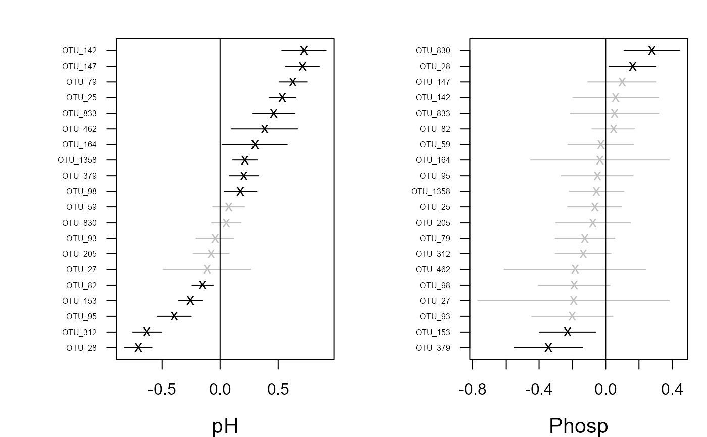
fit <- gllvm(y, X, formula = ~ pH + Phosp, family = poisson())
fit$logL
#> [1] -4004.332
ordiplot(fit)
 coefplot(fit)
 # \donttest{
# Inclusion of structured random row effect
sDesign<-data.frame(Site = microbialdata$Xenv$Site)
fit <- gllvm(y, X, formula = ~ pH + Phosp, family = poisson(),
studyDesign=sDesign, row.eff=~(1|Site))
## Load a dataset from the mvabund package
library(mvabund)
#>
#> Attaching package: 'mvabund'
#> The following object is masked from 'package:gllvm':
#>
#> coefplot
data(antTraits, package = "mvabund")
y <- as.matrix(antTraits$abund)
X <- as.matrix(antTraits$env)
TR <- antTraits$traits
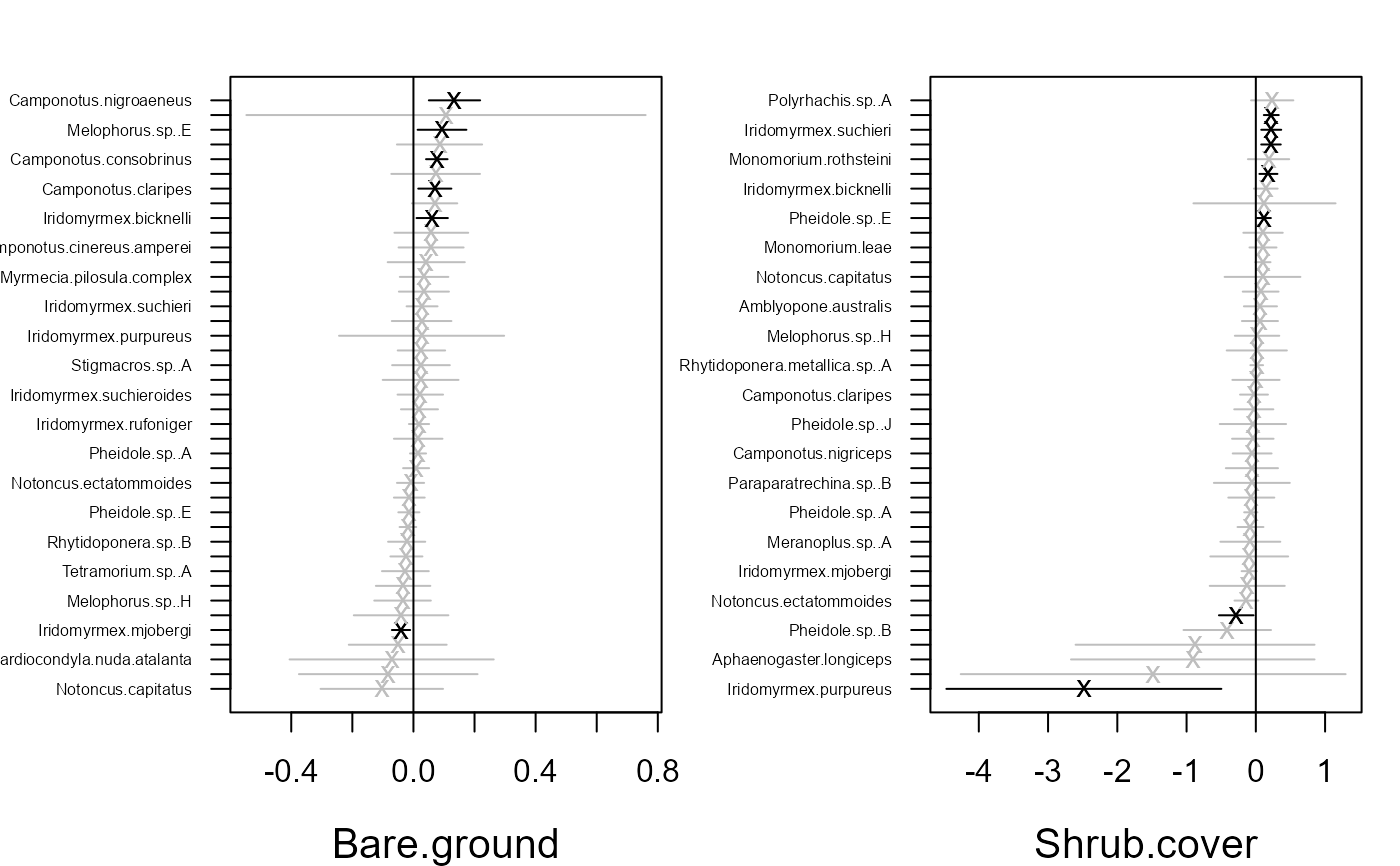
# Fit model with environmental covariates Bare.ground and Shrub.cover
fit <- gllvm(y, X, formula = ~ Bare.ground + Shrub.cover,
family = poisson())
ordiplot(fit)
coefplot.gllvm(fit)
# \donttest{
# Inclusion of structured random row effect
sDesign<-data.frame(Site = microbialdata$Xenv$Site)
fit <- gllvm(y, X, formula = ~ pH + Phosp, family = poisson(),
studyDesign=sDesign, row.eff=~(1|Site))
## Load a dataset from the mvabund package
library(mvabund)
#>
#> Attaching package: 'mvabund'
#> The following object is masked from 'package:gllvm':
#>
#> coefplot
data(antTraits, package = "mvabund")
y <- as.matrix(antTraits$abund)
X <- as.matrix(antTraits$env)
TR <- antTraits$traits
# Fit model with environmental covariates Bare.ground and Shrub.cover
fit <- gllvm(y, X, formula = ~ Bare.ground + Shrub.cover,
family = poisson())
ordiplot(fit)
coefplot.gllvm(fit)

 ## Example 1: Fit model with two unconstrained latent variables
# Using variational approximation:
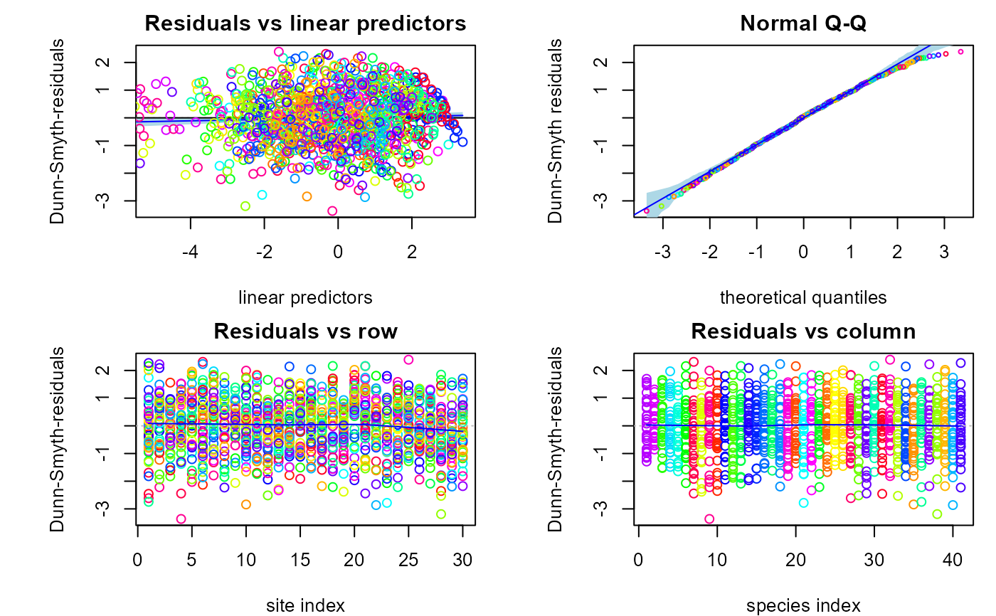
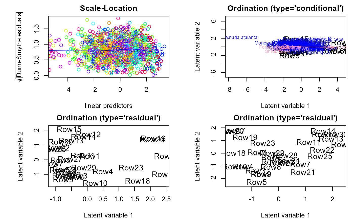
fitv0 <- gllvm(y, family = "negative.binomial", method = "VA")
ordiplot(fitv0)
plot(fitv0, mfrow = c(2,2))
## Example 1: Fit model with two unconstrained latent variables
# Using variational approximation:
fitv0 <- gllvm(y, family = "negative.binomial", method = "VA")
ordiplot(fitv0)
plot(fitv0, mfrow = c(2,2))
 #> Warning: supplied color is neither numeric nor character
 #> Warning: supplied color is neither numeric nor character
summary(fitv0)
#>
#> Call:
#> gllvm(y = y, family = "negative.binomial", method = "VA")
#>
#> Family: negative.binomial
#>
#> AIC: 4056.17 AICc: 4106.324 BIC: 4889.878 LL: -1865.1 df: 163
#>
#> Informed LVs: 0
#> Constrained LVs: 0
#> Unconstrained LVs: 2
#>
#> Formula: ~ 1
#> LV formula: ~ 0
#> Row effect: ~ 1
confint(fitv0)
#> 2.5 % 97.5 %
#> sigma.lv.LV1 -0.103605123 1.85080933
#> sigma.lv.LV2 1.077177540 4.48933510
#> theta.LV1.1 1.000000000 1.00000000
#> theta.LV1.2 -3.375362665 3.62292726
#> theta.LV1.3 -1.024568672 2.94565317
#> theta.LV1.4 -0.679418509 1.55155508
#> theta.LV1.5 -0.461949941 2.15804644
#> theta.LV1.6 -2.600908409 1.44383792
#> theta.LV1.7 -0.924994693 2.07176242
#> theta.LV1.8 -6.335021387 1.22296334
#> theta.LV1.9 -1.593704435 5.82303382
#> theta.LV1.10 -0.559061216 0.96180561
#> theta.LV1.11 -0.995287933 1.38070032
#> theta.LV1.12 -0.703101118 2.72934315
#> theta.LV1.13 -1.200842044 0.16183799
#> theta.LV1.14 -1.111169109 4.02243523
#> theta.LV1.15 -1.109879640 0.73215032
#> theta.LV1.16 -0.654153832 1.49023601
#> theta.LV1.17 -1.785684461 0.71515980
#> theta.LV1.18 -0.929946016 1.19769534
#> theta.LV1.19 -1.537260731 0.27052958
#> theta.LV1.20 -2.295454849 0.40654359
#> theta.LV1.21 -3.204711518 1.07476251
#> theta.LV1.22 -0.368376196 1.81014952
#> theta.LV1.23 -3.334322702 1.20030766
#> theta.LV1.24 -2.427158923 0.63634287
#> theta.LV1.25 -1.106761089 1.40691642
#> theta.LV1.26 -1.365240421 4.42319311
#> theta.LV1.27 -2.057518980 0.22229412
#> theta.LV1.28 -2.567212885 0.76269589
#> theta.LV1.29 -3.329876539 1.97405340
#> theta.LV1.30 -4.802931587 1.56660745
#> theta.LV1.31 -1.016509410 0.15413154
#> theta.LV1.32 -1.695619481 1.09745356
#> theta.LV1.33 -0.212419087 1.10356755
#> theta.LV1.34 -1.671529961 1.01469741
#> theta.LV1.35 -0.597915150 1.34013034
#> theta.LV1.36 -0.987881259 0.19181996
#> theta.LV1.37 -2.777100851 0.48855300
#> theta.LV1.38 -1.882897057 0.67657428
#> theta.LV1.39 -0.525448932 2.41763983
#> theta.LV1.40 -0.375578778 1.19648155
#> theta.LV1.41 -2.479960937 0.61159823
#> theta.LV2.1 0.000000000 0.00000000
#> theta.LV2.2 1.000000000 1.00000000
#> theta.LV2.3 -0.244926341 0.60944662
#> theta.LV2.4 -0.058024771 0.36356423
#> theta.LV2.5 -0.651706006 0.04093951
#> theta.LV2.6 -0.107582504 0.67606584
#> theta.LV2.7 -0.151722964 0.42707987
#> theta.LV2.8 -1.416690092 0.75991192
#> theta.LV2.9 -0.321751487 1.41123762
#> theta.LV2.10 -0.392872328 -0.01049274
#> theta.LV2.11 -0.634803842 -0.10021915
#> theta.LV2.12 -0.503297861 0.43385122
#> theta.LV2.13 -0.161601754 0.20479816
#> theta.LV2.14 -0.221544641 0.87833825
#> theta.LV2.15 -0.471312164 -0.09662699
#> theta.LV2.16 -0.556025943 0.01509584
#> theta.LV2.17 -0.631679769 0.04547439
#> theta.LV2.18 -0.483884182 0.17679198
#> theta.LV2.19 -0.363600013 0.10571700
#> theta.LV2.20 -0.512340060 0.19498832
#> theta.LV2.21 -0.932076760 0.20989970
#> theta.LV2.22 -0.116026293 0.37699844
#> theta.LV2.23 -1.114016591 -0.04366628
#> theta.LV2.24 -0.696499622 0.13926874
#> theta.LV2.25 -0.721257922 0.18283889
#> theta.LV2.26 -0.422604189 0.70790341
#> theta.LV2.27 -0.372660439 0.22420401
#> theta.LV2.28 -0.756108139 0.04819846
#> theta.LV2.29 -1.545154176 0.10764115
#> theta.LV2.30 -0.307275075 0.93014840
#> theta.LV2.31 -0.211031694 0.07090139
#> theta.LV2.32 -0.014484778 0.58033786
#> theta.LV2.33 -0.253862944 0.10709219
#> theta.LV2.34 -0.289127960 0.68818811
#> theta.LV2.35 -0.263434777 0.21007463
#> theta.LV2.36 -0.241972158 0.03942515
#> theta.LV2.37 -0.621233134 0.17246757
#> theta.LV2.38 -0.300912629 0.46344328
#> theta.LV2.39 -0.299116661 0.35709809
#> theta.LV2.40 -0.362541359 0.04883531
#> theta.LV2.41 -0.709337841 0.06374888
#> Intercept.Amblyopone.australis -1.853490627 -0.03146978
#> Intercept.Aphaenogaster.longiceps -6.258629731 -0.31575729
#> Intercept.Camponotus.cinereus.amperei -3.697420812 -0.83559995
#> Intercept.Camponotus.claripes -0.036415394 1.06028791
#> Intercept.Camponotus.consobrinus 0.642102297 1.79316541
#> Intercept.Camponotus.nigriceps -1.679320380 0.47981337
#> Intercept.Camponotus.nigroaeneus -1.317285589 0.23422593
#> Intercept.Cardiocondyla.nuda.atalanta -5.333020236 -0.01397110
#> Intercept.Crematogaster.sp..A -4.740928300 0.10320204
#> Intercept.Heteroponera.sp..A 0.802061269 1.67636391
#> Intercept.Iridomyrmex.bicknelli 0.772365602 1.80407503
#> Intercept.Iridomyrmex.dromus -1.858629719 0.26236864
#> Intercept.Iridomyrmex.mjobergi 0.981615433 1.68321608
#> Intercept.Iridomyrmex.purpureus -1.287468445 1.11343106
#> Intercept.Iridomyrmex.rufoniger 2.021712567 2.70265766
#> Intercept.Iridomyrmex.suchieri -0.135404309 1.04234699
#> Intercept.Iridomyrmex.suchieroides -1.136153120 0.24753984
#> Intercept.Melophorus.sp..E -2.009272680 -0.37476354
#> Intercept.Melophorus.sp..F 0.082415765 0.98211137
#> Intercept.Melophorus.sp..H -1.273684427 0.15974542
#> Intercept.Meranoplus.sp..A -1.455128760 0.64803311
#> Intercept.Monomorium.leae 0.841778667 1.84768435
#> Intercept.Monomorium.rothsteini -0.732316190 1.20871807
#> Intercept.Monomorium.sydneyense -1.321283737 0.40677100
#> Intercept.Myrmecia.pilosula.complex -2.053749665 -0.20212459
#> Intercept.Notoncus.capitatus -2.473090686 0.53518661
#> Intercept.Notoncus.ectatommoides 0.238742753 1.22209016
#> Intercept.Nylanderia.sp..A 0.029632980 1.46946455
#> Intercept.Ochetellus.glaber -3.866770725 -0.21666901
#> Intercept.Paraparatrechina.sp..B -3.312121550 0.27489669
#> Intercept.Pheidole.sp..A 2.092209520 2.54350973
#> Intercept.Pheidole.sp..B -2.030103155 -0.15318951
#> Intercept.Pheidole.sp..E 1.226639097 1.97951051
#> Intercept.Pheidole.sp..J -2.978214611 -0.56714798
#> Intercept.Polyrhachis.sp..A -1.984298751 -0.52860232
#> Intercept.Rhytidoponera.metallica.sp..A 1.772529281 2.27334309
#> Intercept.Rhytidoponera.sp..B -0.397708318 1.09373744
#> Intercept.Solenopsis.sp..A -3.427164156 -0.97579538
#> Intercept.Stigmacros.sp..A -1.091216389 0.51308332
#> Intercept.Tapinoma.sp..A 0.282453416 1.23733490
#> Intercept.Tetramorium.sp..A -0.632172158 0.77827551
#> phi.Amblyopone.australis -0.270744316 1.34951473
#> phi.Aphaenogaster.longiceps -0.211436256 1.00814024
#> phi.Camponotus.cinereus.amperei -1.084013396 2.59065305
#> phi.Camponotus.claripes 0.057458682 1.51932448
#> phi.Camponotus.consobrinus 0.052987973 3.83183156
#> phi.Camponotus.nigriceps -0.061325602 0.51819972
#> phi.Camponotus.nigroaeneus -0.106572767 1.07125854
#> phi.Cardiocondyla.nuda.atalanta -0.070028342 0.42282605
#> phi.Crematogaster.sp..A -0.079407108 0.52843063
#> phi.Heteroponera.sp..A 0.225146177 2.46885155
#> phi.Iridomyrmex.bicknelli -0.118101318 5.03006028
#> phi.Iridomyrmex.dromus -0.066757464 0.56596155
#> phi.Iridomyrmex.mjobergi -0.170198887 4.83897716
#> phi.Iridomyrmex.purpureus 0.009083505 0.42277444
#> phi.Iridomyrmex.rufoniger -0.083810059 19.14608378
#> phi.Iridomyrmex.suchieri -0.154699492 2.35791890
#> phi.Iridomyrmex.suchieroides -0.884451625 4.74668061
#> phi.Melophorus.sp..E -0.832176335 2.32028468
#> phi.Melophorus.sp..F -0.512480593 5.30082254
#> phi.Melophorus.sp..H -0.424024140 3.55517788
#> phi.Meranoplus.sp..A -0.018459555 0.63752743
#> phi.Monomorium.leae 0.248442283 1.69128082
#> phi.Monomorium.rothsteini 0.014823211 2.74656796
#> phi.Monomorium.sydneyense -0.099514155 1.27886013
#> phi.Myrmecia.pilosula.complex -0.365793752 1.37931885
#> phi.Notoncus.capitatus -0.041835629 0.38612708
#> phi.Notoncus.ectatommoides -0.084173806 4.06966012
#> phi.Nylanderia.sp..A 0.107368056 1.41124120
#> phi.Ochetellus.glaber -0.188675663 1.06100099
#> phi.Paraparatrechina.sp..B -0.063989465 0.30184580
#> phi.Pheidole.sp..A -1.416707130 20.56551585
#> phi.Pheidole.sp..B -0.348482502 1.33681298
#> phi.Pheidole.sp..E 0.320677934 2.69259269
#> phi.Pheidole.sp..J -0.276763965 0.79871876
#> phi.Polyrhachis.sp..A -7.667384113 15.05304906
#> phi.Rhytidoponera.metallica.sp..A -0.858531555 15.09466611
#> phi.Rhytidoponera.sp..B 0.003911047 1.35235632
#> phi.Solenopsis.sp..A -1.918670065 4.16909826
#> phi.Stigmacros.sp..A -0.028717976 1.05055230
#> phi.Tapinoma.sp..A 0.106426751 2.27942789
#> phi.Tetramorium.sp..A -0.300540655 3.63477523
## Example 1a: Fit concurrent ordination model with two latent variables and with
# quadratic response model
# We scale and centre the predictors to improve convergence
fity1 <- gllvm(y, X = scale(X), family = "negative.binomial",
num.lv.c=2, method="VA")
ordiplot(fity1, biplot = TRUE)
#'## Example 1b: Fit constrained ordination model with two latent variables and with
# random canonical coefficients
fity2 <- gllvm(y, X = scale(X), family = "negative.binomial",
num.RR=2, randomB="LV", method="VA")
#> Warning: 54 parameter(s) have negative variance estimates (lambda x53, sigmab_lv x1). The model likely has not converged - consider re-fitting.
# Using Laplace approximation: (this line may take about 30 sec to run)
fitl0 <- gllvm(y, family = "negative.binomial", method = "LA")
#> Warning: 3 parameter(s) have negative variance estimates (lg_phi x3). The model likely has not converged - consider re-fitting.
ordiplot(fitl0)
# Poisson family:
fit.p <- gllvm(y, family = poisson(), method = "LA")
ordiplot(fit.p)
#> Warning: supplied color is neither numeric nor character
summary(fitv0)
#>
#> Call:
#> gllvm(y = y, family = "negative.binomial", method = "VA")
#>
#> Family: negative.binomial
#>
#> AIC: 4056.17 AICc: 4106.324 BIC: 4889.878 LL: -1865.1 df: 163
#>
#> Informed LVs: 0
#> Constrained LVs: 0
#> Unconstrained LVs: 2
#>
#> Formula: ~ 1
#> LV formula: ~ 0
#> Row effect: ~ 1
confint(fitv0)
#> 2.5 % 97.5 %
#> sigma.lv.LV1 -0.103605123 1.85080933
#> sigma.lv.LV2 1.077177540 4.48933510
#> theta.LV1.1 1.000000000 1.00000000
#> theta.LV1.2 -3.375362665 3.62292726
#> theta.LV1.3 -1.024568672 2.94565317
#> theta.LV1.4 -0.679418509 1.55155508
#> theta.LV1.5 -0.461949941 2.15804644
#> theta.LV1.6 -2.600908409 1.44383792
#> theta.LV1.7 -0.924994693 2.07176242
#> theta.LV1.8 -6.335021387 1.22296334
#> theta.LV1.9 -1.593704435 5.82303382
#> theta.LV1.10 -0.559061216 0.96180561
#> theta.LV1.11 -0.995287933 1.38070032
#> theta.LV1.12 -0.703101118 2.72934315
#> theta.LV1.13 -1.200842044 0.16183799
#> theta.LV1.14 -1.111169109 4.02243523
#> theta.LV1.15 -1.109879640 0.73215032
#> theta.LV1.16 -0.654153832 1.49023601
#> theta.LV1.17 -1.785684461 0.71515980
#> theta.LV1.18 -0.929946016 1.19769534
#> theta.LV1.19 -1.537260731 0.27052958
#> theta.LV1.20 -2.295454849 0.40654359
#> theta.LV1.21 -3.204711518 1.07476251
#> theta.LV1.22 -0.368376196 1.81014952
#> theta.LV1.23 -3.334322702 1.20030766
#> theta.LV1.24 -2.427158923 0.63634287
#> theta.LV1.25 -1.106761089 1.40691642
#> theta.LV1.26 -1.365240421 4.42319311
#> theta.LV1.27 -2.057518980 0.22229412
#> theta.LV1.28 -2.567212885 0.76269589
#> theta.LV1.29 -3.329876539 1.97405340
#> theta.LV1.30 -4.802931587 1.56660745
#> theta.LV1.31 -1.016509410 0.15413154
#> theta.LV1.32 -1.695619481 1.09745356
#> theta.LV1.33 -0.212419087 1.10356755
#> theta.LV1.34 -1.671529961 1.01469741
#> theta.LV1.35 -0.597915150 1.34013034
#> theta.LV1.36 -0.987881259 0.19181996
#> theta.LV1.37 -2.777100851 0.48855300
#> theta.LV1.38 -1.882897057 0.67657428
#> theta.LV1.39 -0.525448932 2.41763983
#> theta.LV1.40 -0.375578778 1.19648155
#> theta.LV1.41 -2.479960937 0.61159823
#> theta.LV2.1 0.000000000 0.00000000
#> theta.LV2.2 1.000000000 1.00000000
#> theta.LV2.3 -0.244926341 0.60944662
#> theta.LV2.4 -0.058024771 0.36356423
#> theta.LV2.5 -0.651706006 0.04093951
#> theta.LV2.6 -0.107582504 0.67606584
#> theta.LV2.7 -0.151722964 0.42707987
#> theta.LV2.8 -1.416690092 0.75991192
#> theta.LV2.9 -0.321751487 1.41123762
#> theta.LV2.10 -0.392872328 -0.01049274
#> theta.LV2.11 -0.634803842 -0.10021915
#> theta.LV2.12 -0.503297861 0.43385122
#> theta.LV2.13 -0.161601754 0.20479816
#> theta.LV2.14 -0.221544641 0.87833825
#> theta.LV2.15 -0.471312164 -0.09662699
#> theta.LV2.16 -0.556025943 0.01509584
#> theta.LV2.17 -0.631679769 0.04547439
#> theta.LV2.18 -0.483884182 0.17679198
#> theta.LV2.19 -0.363600013 0.10571700
#> theta.LV2.20 -0.512340060 0.19498832
#> theta.LV2.21 -0.932076760 0.20989970
#> theta.LV2.22 -0.116026293 0.37699844
#> theta.LV2.23 -1.114016591 -0.04366628
#> theta.LV2.24 -0.696499622 0.13926874
#> theta.LV2.25 -0.721257922 0.18283889
#> theta.LV2.26 -0.422604189 0.70790341
#> theta.LV2.27 -0.372660439 0.22420401
#> theta.LV2.28 -0.756108139 0.04819846
#> theta.LV2.29 -1.545154176 0.10764115
#> theta.LV2.30 -0.307275075 0.93014840
#> theta.LV2.31 -0.211031694 0.07090139
#> theta.LV2.32 -0.014484778 0.58033786
#> theta.LV2.33 -0.253862944 0.10709219
#> theta.LV2.34 -0.289127960 0.68818811
#> theta.LV2.35 -0.263434777 0.21007463
#> theta.LV2.36 -0.241972158 0.03942515
#> theta.LV2.37 -0.621233134 0.17246757
#> theta.LV2.38 -0.300912629 0.46344328
#> theta.LV2.39 -0.299116661 0.35709809
#> theta.LV2.40 -0.362541359 0.04883531
#> theta.LV2.41 -0.709337841 0.06374888
#> Intercept.Amblyopone.australis -1.853490627 -0.03146978
#> Intercept.Aphaenogaster.longiceps -6.258629731 -0.31575729
#> Intercept.Camponotus.cinereus.amperei -3.697420812 -0.83559995
#> Intercept.Camponotus.claripes -0.036415394 1.06028791
#> Intercept.Camponotus.consobrinus 0.642102297 1.79316541
#> Intercept.Camponotus.nigriceps -1.679320380 0.47981337
#> Intercept.Camponotus.nigroaeneus -1.317285589 0.23422593
#> Intercept.Cardiocondyla.nuda.atalanta -5.333020236 -0.01397110
#> Intercept.Crematogaster.sp..A -4.740928300 0.10320204
#> Intercept.Heteroponera.sp..A 0.802061269 1.67636391
#> Intercept.Iridomyrmex.bicknelli 0.772365602 1.80407503
#> Intercept.Iridomyrmex.dromus -1.858629719 0.26236864
#> Intercept.Iridomyrmex.mjobergi 0.981615433 1.68321608
#> Intercept.Iridomyrmex.purpureus -1.287468445 1.11343106
#> Intercept.Iridomyrmex.rufoniger 2.021712567 2.70265766
#> Intercept.Iridomyrmex.suchieri -0.135404309 1.04234699
#> Intercept.Iridomyrmex.suchieroides -1.136153120 0.24753984
#> Intercept.Melophorus.sp..E -2.009272680 -0.37476354
#> Intercept.Melophorus.sp..F 0.082415765 0.98211137
#> Intercept.Melophorus.sp..H -1.273684427 0.15974542
#> Intercept.Meranoplus.sp..A -1.455128760 0.64803311
#> Intercept.Monomorium.leae 0.841778667 1.84768435
#> Intercept.Monomorium.rothsteini -0.732316190 1.20871807
#> Intercept.Monomorium.sydneyense -1.321283737 0.40677100
#> Intercept.Myrmecia.pilosula.complex -2.053749665 -0.20212459
#> Intercept.Notoncus.capitatus -2.473090686 0.53518661
#> Intercept.Notoncus.ectatommoides 0.238742753 1.22209016
#> Intercept.Nylanderia.sp..A 0.029632980 1.46946455
#> Intercept.Ochetellus.glaber -3.866770725 -0.21666901
#> Intercept.Paraparatrechina.sp..B -3.312121550 0.27489669
#> Intercept.Pheidole.sp..A 2.092209520 2.54350973
#> Intercept.Pheidole.sp..B -2.030103155 -0.15318951
#> Intercept.Pheidole.sp..E 1.226639097 1.97951051
#> Intercept.Pheidole.sp..J -2.978214611 -0.56714798
#> Intercept.Polyrhachis.sp..A -1.984298751 -0.52860232
#> Intercept.Rhytidoponera.metallica.sp..A 1.772529281 2.27334309
#> Intercept.Rhytidoponera.sp..B -0.397708318 1.09373744
#> Intercept.Solenopsis.sp..A -3.427164156 -0.97579538
#> Intercept.Stigmacros.sp..A -1.091216389 0.51308332
#> Intercept.Tapinoma.sp..A 0.282453416 1.23733490
#> Intercept.Tetramorium.sp..A -0.632172158 0.77827551
#> phi.Amblyopone.australis -0.270744316 1.34951473
#> phi.Aphaenogaster.longiceps -0.211436256 1.00814024
#> phi.Camponotus.cinereus.amperei -1.084013396 2.59065305
#> phi.Camponotus.claripes 0.057458682 1.51932448
#> phi.Camponotus.consobrinus 0.052987973 3.83183156
#> phi.Camponotus.nigriceps -0.061325602 0.51819972
#> phi.Camponotus.nigroaeneus -0.106572767 1.07125854
#> phi.Cardiocondyla.nuda.atalanta -0.070028342 0.42282605
#> phi.Crematogaster.sp..A -0.079407108 0.52843063
#> phi.Heteroponera.sp..A 0.225146177 2.46885155
#> phi.Iridomyrmex.bicknelli -0.118101318 5.03006028
#> phi.Iridomyrmex.dromus -0.066757464 0.56596155
#> phi.Iridomyrmex.mjobergi -0.170198887 4.83897716
#> phi.Iridomyrmex.purpureus 0.009083505 0.42277444
#> phi.Iridomyrmex.rufoniger -0.083810059 19.14608378
#> phi.Iridomyrmex.suchieri -0.154699492 2.35791890
#> phi.Iridomyrmex.suchieroides -0.884451625 4.74668061
#> phi.Melophorus.sp..E -0.832176335 2.32028468
#> phi.Melophorus.sp..F -0.512480593 5.30082254
#> phi.Melophorus.sp..H -0.424024140 3.55517788
#> phi.Meranoplus.sp..A -0.018459555 0.63752743
#> phi.Monomorium.leae 0.248442283 1.69128082
#> phi.Monomorium.rothsteini 0.014823211 2.74656796
#> phi.Monomorium.sydneyense -0.099514155 1.27886013
#> phi.Myrmecia.pilosula.complex -0.365793752 1.37931885
#> phi.Notoncus.capitatus -0.041835629 0.38612708
#> phi.Notoncus.ectatommoides -0.084173806 4.06966012
#> phi.Nylanderia.sp..A 0.107368056 1.41124120
#> phi.Ochetellus.glaber -0.188675663 1.06100099
#> phi.Paraparatrechina.sp..B -0.063989465 0.30184580
#> phi.Pheidole.sp..A -1.416707130 20.56551585
#> phi.Pheidole.sp..B -0.348482502 1.33681298
#> phi.Pheidole.sp..E 0.320677934 2.69259269
#> phi.Pheidole.sp..J -0.276763965 0.79871876
#> phi.Polyrhachis.sp..A -7.667384113 15.05304906
#> phi.Rhytidoponera.metallica.sp..A -0.858531555 15.09466611
#> phi.Rhytidoponera.sp..B 0.003911047 1.35235632
#> phi.Solenopsis.sp..A -1.918670065 4.16909826
#> phi.Stigmacros.sp..A -0.028717976 1.05055230
#> phi.Tapinoma.sp..A 0.106426751 2.27942789
#> phi.Tetramorium.sp..A -0.300540655 3.63477523
## Example 1a: Fit concurrent ordination model with two latent variables and with
# quadratic response model
# We scale and centre the predictors to improve convergence
fity1 <- gllvm(y, X = scale(X), family = "negative.binomial",
num.lv.c=2, method="VA")
ordiplot(fity1, biplot = TRUE)
#'## Example 1b: Fit constrained ordination model with two latent variables and with
# random canonical coefficients
fity2 <- gllvm(y, X = scale(X), family = "negative.binomial",
num.RR=2, randomB="LV", method="VA")
#> Warning: 54 parameter(s) have negative variance estimates (lambda x53, sigmab_lv x1). The model likely has not converged - consider re-fitting.
# Using Laplace approximation: (this line may take about 30 sec to run)
fitl0 <- gllvm(y, family = "negative.binomial", method = "LA")
#> Warning: 3 parameter(s) have negative variance estimates (lg_phi x3). The model likely has not converged - consider re-fitting.
ordiplot(fitl0)
# Poisson family:
fit.p <- gllvm(y, family = poisson(), method = "LA")
ordiplot(fit.p)
 # Use poisson model as a starting parameters for ZIP-model, this line
# may take few minutes to run
fit.z <- gllvm(y, family = "ZIP", method = "LA",
control.start = list(start.fit = fit.p))
#> Warning: 18 parameter(s) have negative variance estimates (b x3, lambda x12, lg_phi x3). The model likely has not converged - consider re-fitting.
#> Warning: Determinant of the variance-covariance matix is zero. Please double check your model for e.g. overfitting or lack of convergence.
ordiplot(fit.z)
## Example 2: gllvm with environmental variables
# Fit model with two latent variables and all environmental covariates,
fitvX <- gllvm(formula = y ~ X, family = "negative.binomial")
ordiplot(fitvX, biplot = TRUE)
coefplot.gllvm(fitvX)
# Use poisson model as a starting parameters for ZIP-model, this line
# may take few minutes to run
fit.z <- gllvm(y, family = "ZIP", method = "LA",
control.start = list(start.fit = fit.p))
#> Warning: 18 parameter(s) have negative variance estimates (b x3, lambda x12, lg_phi x3). The model likely has not converged - consider re-fitting.
#> Warning: Determinant of the variance-covariance matix is zero. Please double check your model for e.g. overfitting or lack of convergence.
ordiplot(fit.z)
## Example 2: gllvm with environmental variables
# Fit model with two latent variables and all environmental covariates,
fitvX <- gllvm(formula = y ~ X, family = "negative.binomial")
ordiplot(fitvX, biplot = TRUE)
coefplot.gllvm(fitvX)

 # Fit model with environmental covariates Bare.ground and Shrub.cover
fitvX2 <- gllvm(y, X, formula = ~ Bare.ground + Shrub.cover,
family = "negative.binomial")
ordiplot(fitvX2)
coefplot.gllvm(fitvX2)
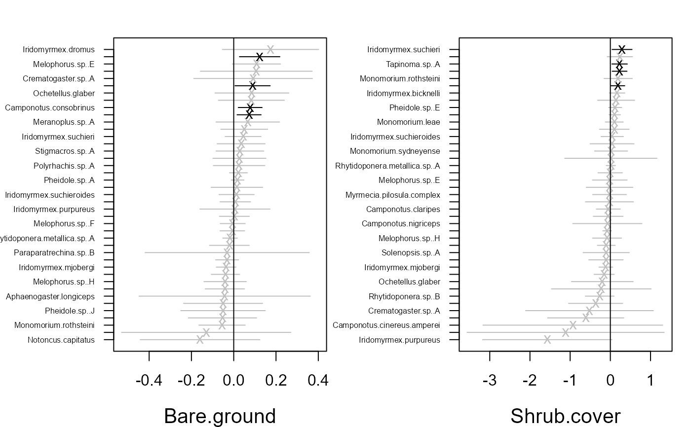
# Fit model with environmental covariates Bare.ground and Shrub.cover
fitvX2 <- gllvm(y, X, formula = ~ Bare.ground + Shrub.cover,
family = "negative.binomial")
ordiplot(fitvX2)
coefplot.gllvm(fitvX2)

 # Use 5 initial runs and pick the best one
fitvX_5 <- gllvm(y, X, formula = ~ Bare.ground + Shrub.cover,
family = "negative.binomial", control.start=list(n.init = 5, jitter.var = 0.1))
ordiplot(fitvX_5)
coefplot.gllvm(fitvX_5)
# Use 5 initial runs and pick the best one
fitvX_5 <- gllvm(y, X, formula = ~ Bare.ground + Shrub.cover,
family = "negative.binomial", control.start=list(n.init = 5, jitter.var = 0.1))
ordiplot(fitvX_5)
coefplot.gllvm(fitvX_5)

 ## Example 3: Data in long format
# Reshape data to long format:
datalong <- reshape(data.frame(cbind(y,X)), direction = "long",
varying = colnames(y), v.names = "y")
head(datalong)
#> Bare.ground Canopy.cover Shrub.cover Volume.lying.CWD Feral.mammal.dung
#> 1.1 9.00 3.5 0.50 0.03253833 0.20
#> 2.1 6.00 0.0 0.00 0.01202944 0.65
#> 3.1 9.25 0.0 8.10 0.00804195 0.00
#> 4.1 23.25 0.0 0.25 0.00000000 0.20
#> 5.1 8.75 0.0 3.35 0.00993944 0.35
#> 6.1 32.25 0.0 0.00 0.03142221 1.00
#> time y id
#> 1.1 1 0 1
#> 2.1 1 0 2
#> 3.1 1 0 3
#> 4.1 1 4 4
#> 5.1 1 2 5
#> 6.1 1 0 6
fitvLong <- gllvm(data = datalong, formula = y ~ Bare.ground + Shrub.cover,
family = "negative.binomial")
## Example 4: Fourth corner model
# Fit fourth corner model with two latent variables
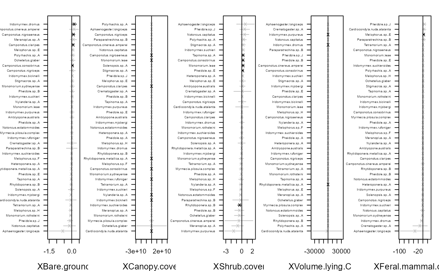
fitF1 <- gllvm(y = y, X = X, TR = TR, family = "negative.binomial")
coefplot.gllvm(fitF1)
## Example 3: Data in long format
# Reshape data to long format:
datalong <- reshape(data.frame(cbind(y,X)), direction = "long",
varying = colnames(y), v.names = "y")
head(datalong)
#> Bare.ground Canopy.cover Shrub.cover Volume.lying.CWD Feral.mammal.dung
#> 1.1 9.00 3.5 0.50 0.03253833 0.20
#> 2.1 6.00 0.0 0.00 0.01202944 0.65
#> 3.1 9.25 0.0 8.10 0.00804195 0.00
#> 4.1 23.25 0.0 0.25 0.00000000 0.20
#> 5.1 8.75 0.0 3.35 0.00993944 0.35
#> 6.1 32.25 0.0 0.00 0.03142221 1.00
#> time y id
#> 1.1 1 0 1
#> 2.1 1 0 2
#> 3.1 1 0 3
#> 4.1 1 4 4
#> 5.1 1 2 5
#> 6.1 1 0 6
fitvLong <- gllvm(data = datalong, formula = y ~ Bare.ground + Shrub.cover,
family = "negative.binomial")
## Example 4: Fourth corner model
# Fit fourth corner model with two latent variables
fitF1 <- gllvm(y = y, X = X, TR = TR, family = "negative.binomial")
coefplot.gllvm(fitF1)
 # Fourth corner can be plotted also with next lines
#fourth = fitF1$fourth.corner
#library(lattice)
#a = max( abs(fourth) )
#colort = colorRampPalette(c("blue","white","red"))
#plot.4th = levelplot(t(as.matrix(fourth)), xlab = "Environmental Variables",
# ylab = "Species traits", col.regions = colort(100),
# at = seq( -a, a, length = 100), scales = list( x = list(rot = 45)))
#print(plot.4th)
# Specify model using formula
fitF2 <- gllvm(y = y, X = X, TR = TR,
formula = ~ Bare.ground + Canopy.cover * (Pilosity + Webers.length),
family = "negative.binomial")
ordiplot(fitF2)
# Fourth corner can be plotted also with next lines
#fourth = fitF1$fourth.corner
#library(lattice)
#a = max( abs(fourth) )
#colort = colorRampPalette(c("blue","white","red"))
#plot.4th = levelplot(t(as.matrix(fourth)), xlab = "Environmental Variables",
# ylab = "Species traits", col.regions = colort(100),
# at = seq( -a, a, length = 100), scales = list( x = list(rot = 45)))
#print(plot.4th)
# Specify model using formula
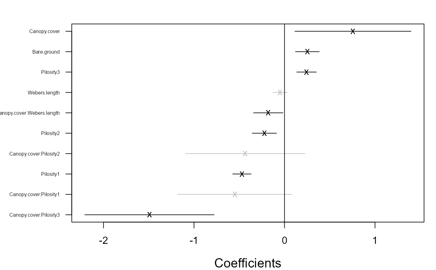
fitF2 <- gllvm(y = y, X = X, TR = TR,
formula = ~ Bare.ground + Canopy.cover * (Pilosity + Webers.length),
family = "negative.binomial")
ordiplot(fitF2)
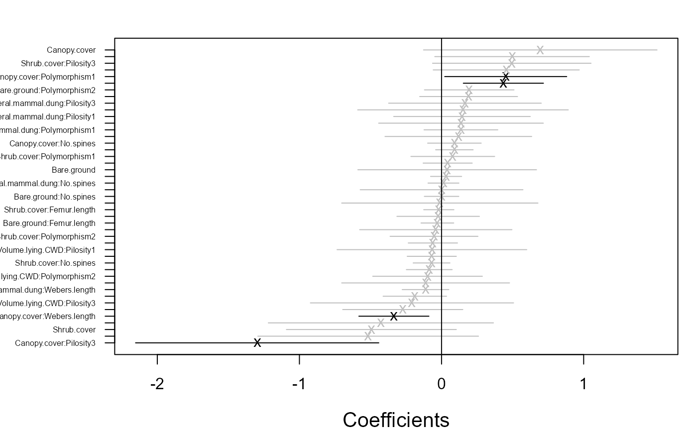
 coefplot.gllvm(fitF2)
 ## Include species specific random slopes to the fourth corner model
fitF3 <- gllvm(y = y, X = X, TR = TR,
formula = ~ Bare.ground + Canopy.cover * (Pilosity + Webers.length),
family = "negative.binomial", randomX = ~ Bare.ground + Canopy.cover,
control.start = list(n.init = 3))
#> Warning: 2 parameter(s) have negative variance estimates (sigmaB x1, sigmaij x1). Standard errors are 0 for these. The model likely has not converged - consider re-fitting.
ordiplot(fitF3)
## Include species specific random slopes to the fourth corner model
fitF3 <- gllvm(y = y, X = X, TR = TR,
formula = ~ Bare.ground + Canopy.cover * (Pilosity + Webers.length),
family = "negative.binomial", randomX = ~ Bare.ground + Canopy.cover,
control.start = list(n.init = 3))
#> Warning: 2 parameter(s) have negative variance estimates (sigmaB x1, sigmaij x1). Standard errors are 0 for these. The model likely has not converged - consider re-fitting.
ordiplot(fitF3)
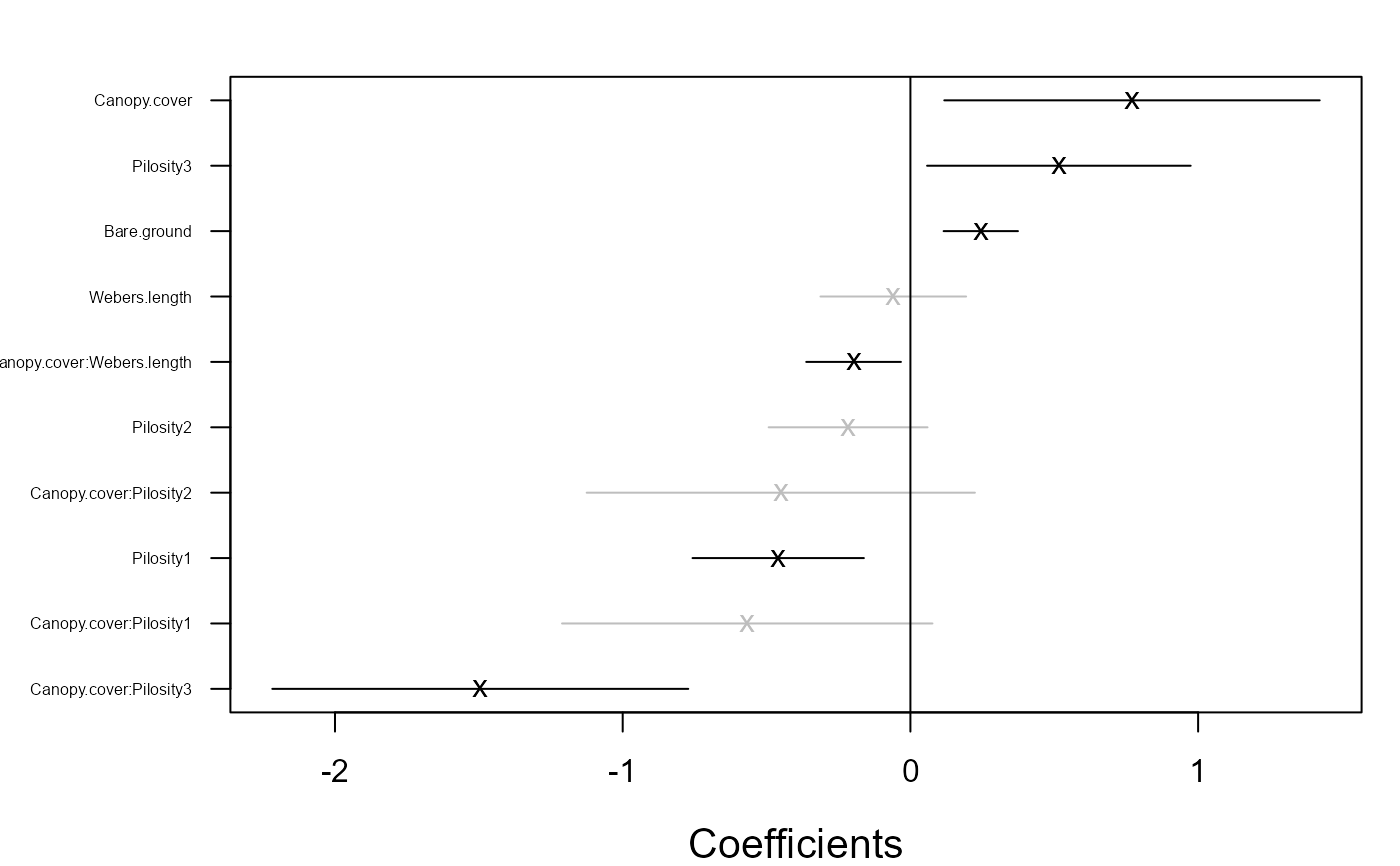
 coefplot.gllvm(fitF3)
 ## Example 5: Fit Tweedie model
# Load coral data
data(tikus)
ycoral <- tikus$abund
# Let's consider only years 1981 and 1983
ycoral <- ycoral[((tikus$x$time == 81) + (tikus$x$time == 83)) > 0, ]
# Exclude species which have observed at less than 4 sites
ycoral <- ycoral[-17, (colSums(ycoral > 0) > 4)]
# Fit Tweedie model for coral data (this line may take few minutes to run)
fit.twe <- gllvm(y = ycoral, family = "tweedie", method = "EVA", seed=111)
#> Warning: method L-BFGS-B uses 'factr' (and 'pgtol') instead of 'reltol' and 'abstol'
fit.twe
#> Call:
#> gllvm(y = ycoral, family = "tweedie", method = "EVA", seed = 111)
#> family:
#> [1] "tweedie"
#> method:
#> [1] "EVA"
#>
#> log-likelihood: -631.5667
#> Residual degrees of freedom: 271
#> AIC: 1405.133
#> AICc: 1443
#> BIC: 1677.405
## Example 6: Random row effects
fitRand <- gllvm(y, family = "negative.binomial", row.eff = "random")
ordiplot(fitRand, biplot = TRUE)
## Example 5: Fit Tweedie model
# Load coral data
data(tikus)
ycoral <- tikus$abund
# Let's consider only years 1981 and 1983
ycoral <- ycoral[((tikus$x$time == 81) + (tikus$x$time == 83)) > 0, ]
# Exclude species which have observed at less than 4 sites
ycoral <- ycoral[-17, (colSums(ycoral > 0) > 4)]
# Fit Tweedie model for coral data (this line may take few minutes to run)
fit.twe <- gllvm(y = ycoral, family = "tweedie", method = "EVA", seed=111)
#> Warning: method L-BFGS-B uses 'factr' (and 'pgtol') instead of 'reltol' and 'abstol'
fit.twe
#> Call:
#> gllvm(y = ycoral, family = "tweedie", method = "EVA", seed = 111)
#> family:
#> [1] "tweedie"
#> method:
#> [1] "EVA"
#>
#> log-likelihood: -631.5667
#> Residual degrees of freedom: 271
#> AIC: 1405.133
#> AICc: 1443
#> BIC: 1677.405
## Example 6: Random row effects
fitRand <- gllvm(y, family = "negative.binomial", row.eff = "random")
ordiplot(fitRand, biplot = TRUE)
 # }
# }