Plot covariate coefficients and confidence intervals

Plots covariate coefficients and their confidence intervals.

# S3 method for gllvm
coefplot(
  object,
  y.label = TRUE,
  which.Xcoef = NULL,
  order = TRUE,
  cex.ylab = 0.5,
  cex.xlab = 1.3,
  mfrow = NULL,
  mar = c(4, 6, 2, 1),
  xlim.list = NULL,
  ...
)

Arguments

object: an object of class 'gllvm'.
y.label: logical, if TRUE (default) colnames of y with respect to coefficients are added to plot.
which.Xcoef: vector indicating which covariate coefficients will be plotted. Can be vector of covariate names or numbers. Default is NULL when all covariate coefficients are plotted.
order: logical, whether or not coefficients are ordered, defaults to TRUE.
cex.ylab: the magnification to be used for axis annotation relative to the current setting of cex.
cex.xlab: the magnification to be used for axis annotation.
mfrow: same as mfrow in par. If NULL (default) it is determined automatically.
mar: vector of length 4, which defines the margin sizes: c(bottom, left, top, right). Defaults to c(4,5,2,1).
xlim.list: list of vectors with length of two to define the intervals for an x axis in each covariate plot. Defaults to NULL when the interval is defined by the range of point estimates and confidence intervals
...: additional graphical arguments.

Author

Jenni Niku <jenni.m.e.niku@jyu.fi>, Francis K.C. Hui, Sara Taskinen, Bert van der Veen

Examples

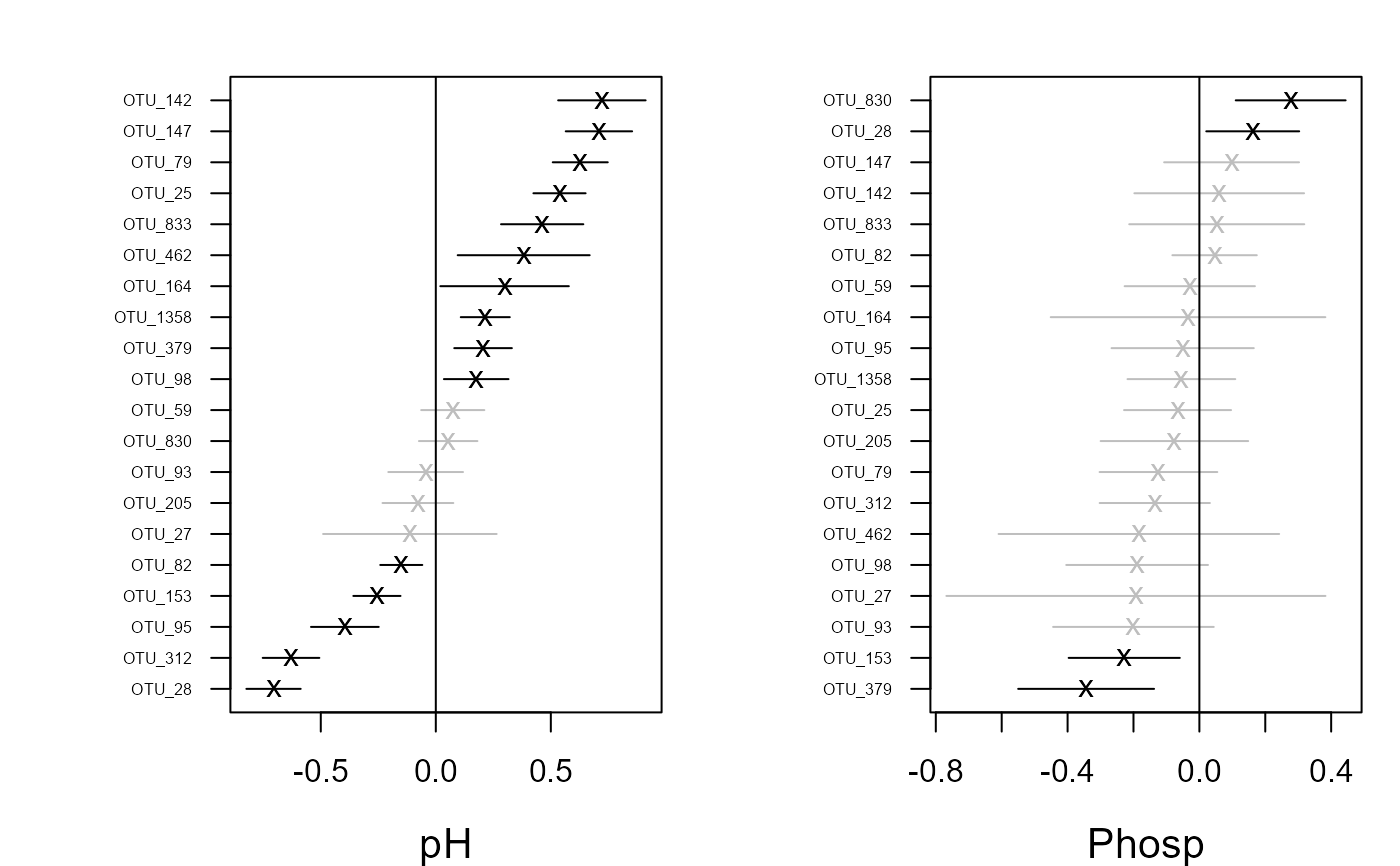
# Extract subset of the microbial data to be used as an example
data(microbialdata)
X <- microbialdata$Xenv
y <- microbialdata$Y[, order(colMeans(microbialdata$Y > 0), 
                     decreasing = TRUE)[21:40]]
fit <- gllvm(y, X, formula = ~ pH + Phosp, family = poisson())
coefplot(fit)

if (FALSE) {
## Load a dataset from the mvabund package
data(antTraits)
y <- as.matrix(antTraits$abund)
X <- as.matrix(antTraits$env)
# Fit model with environmental covariates
fit <- gllvm(y, X, formula = ~ Bare.ground + Shrub.cover,
            family = poisson())
coefplot.gllvm(fit)

# Fit model with all environmental covariates
fitx <- gllvm(y, X, family = "negative.binomial")
coefplot(fitx, mfrow = c(3,2))
coefplot(fitx, which.Xcoef = 1:2)

# Fit gllvm model with environmental and trait covariates
TR <- antTraits$traits
fitT <- gllvm(y = y, X = X, TR = TR, family = "negative.binomial")
coefplot(fitT)

# Fit  gllvm model with environmental covariances and reduced rank
fitRR <- gllvm(y = y, X = X, num.RR = 2, family = "negative.binomial")
coefplot(fitRR)
}