Predict species richness from a gllvm object

Obtains predictions from a fitted generalized linear latent variable model object.

# S3 method for class 'gllvm'
predictSR(
  object,
  spp = NULL,
  expected = "mean",
  se.fit = 1000,
  level = 1,
  ci = "expected",
  alpha = 0.95,
  seed = 42,
  return.pred = FALSE,
  batch = NULL,
  ...
)

Arguments

object: an object of class 'gllvm'.
spp: index vector, defaults to NULL. If omitted, returns a prediction with all species in the data.
expected: character, defaults to "mean", in which case the returned measure of central tendency for species richness is the Poisson-Binomial expectation. Alternatively can be "mode".
se.fit: integer or logical, defaults to 1000. Number of simulations for confidence interval. No confidence interval is returned when set to FALSE.
level: specification for how to predict. Level one (level = 1) attempts to use the predicted site scores from variational approximations or laplace approximation or given site scores in newLV. Level 0 sets the latent variable to zero. Defaults to 1.
ci: character vector, defaults to "expected" but can also be "pmf" or both. If "pmf" provides CI on the whole pmf prediction.
alpha: numeric between 0 and 1, defaults to 0.95. Confidence level of the prediction.
seed: numeric, defaults to 42. Seed for the simulation of the confidence interval.
return.pred: logical, defaults to FALSE. Returns the point-estimate results from "predict.gllvm".
batch: integer or NULL, defaults to 200. If provided, species predictions needed to calculate richness are processed in chunks of this size per simulation draw, reducing peak memory at the cost of more predict calls. NULL processes all (selected) species in one call.
...: arguments passed to "predict.gllvm".

Value

An object of class "predictSR.gllvm" with the following components:

predicted: a list with the predicted Poisson-Binomial distribution as "fit", a matrix of dimension sites by length(SR) with columns named "SR_0", "SR_1", and so on, and, if se.fit is not FALSE and "pmf" %in% ci, the simulated lower and upper confidence bounds "lower" and "upper" (both matrices of the same dimension).
expected: a list with the predicted mean or mode for species richness as "fit", a vector of length \(n\), and, if se.fit is not FALSE and "expected" %in% ci, the simulated lower and upper confidence bounds "lower" and "upper" (both vectors of length \(n\)).
observed: the observed species richness of the data, a vector of length \(n\).
predict.gllvm: only present if return.pred = TRUE; a list with the species-specific predictions from "predict.gllvm".
spp: the indices of the species that richness was calculated for.

Details

This function returns probabilities of richness for species richness from gllvm objects, by first calling "predict.gllvm", and following by predicting from a Poisson-Binomial distribution for richness. The distribution for species richness follows from a sum of binary responses (i.e., occurrence), and is naturally extended to non-normal data types as the probability to get a non-zero observation. Especially with many species and rows, the calculation may take a while.

With expected = "mode" the mode of the Poisson-Binomial distribution is determined from its mean \(\mu\), following Darroch (1964). The distribution can be bimodal with modes \(\lfloor \mu \rfloor\) and \(\lfloor \mu \rfloor + 1\), in which case the lower of the two is returned.

Note

The point estimate ("fit") can sometimes be outside of the simulated intervals when the model fit is poor, the standard errors of parameter estimates are on very different scales, or the number of simulations is too low. Try either 1) scaling and centering covariates in the model, 2) repeatedly refitting the model (see the n.init argument in "gllvm") to find a better set of starting values and improve the fit, or 3) increasing the number of simulations via 'n.init'.

References

Darroch, J. N. (1964). On the distribution of the number of successes in independent trials. The Annals of Mathematical Statistics, 35, 1317-1321.

Author

Bert van der Veen

Examples

# \donttest{
# Load a dataset from the mvabund package
data(spider, package = "mvabund")
y <- as.matrix(spider$abund)
X <- scale(spider$x)
# Fit gllvm model
fit <- gllvm(y = y, X, formula = ~soil.dry, family = poisson())
# Fitted values
newX = data.frame(soil.dry = seq(min(X[,"soil.dry"]),
                 max(X[,"soil.dry"]),length.out=100))
predSR <- predictSR(fit, newX = newX, level = 0)

# Visualize the results
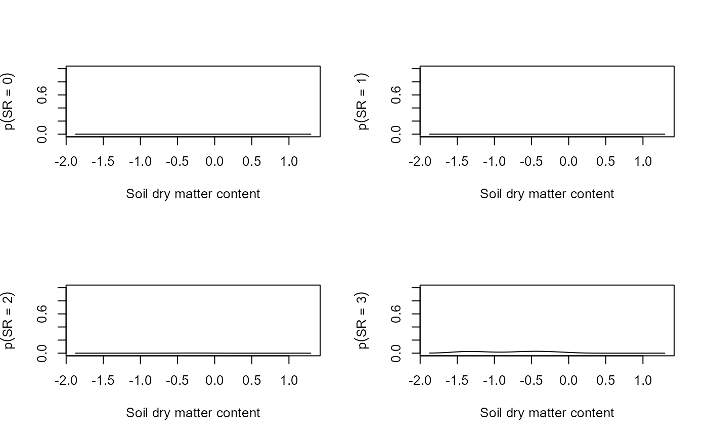
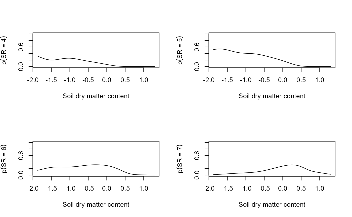
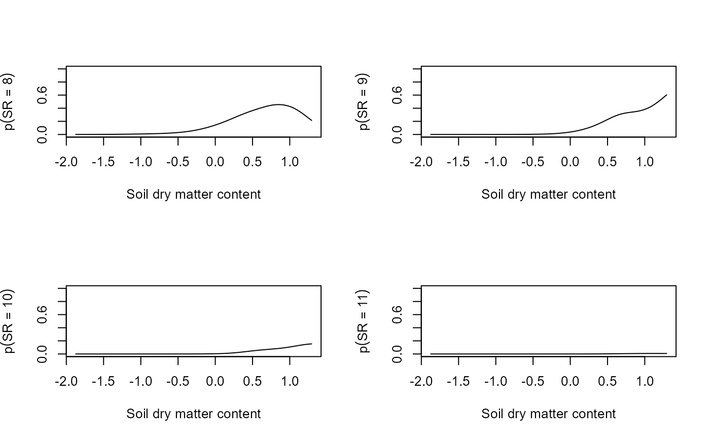
par(mfrow = c(2,2))
for(i in 0:ncol(fit$y)){
plot(x = newX$soil.dry, y = predSR$predicted$fit[,i+1], 
     xlab = "Soil dry matter content", 
     ylab = bquote(p(SR == .(i))), type = "l", ylim = c(0,1))
}




# }